biharmonicSplineInterpolation

Below is a demonstration of the features of the biharmonicSplineInterpolation function

Contents

clear; close all; clc;

Syntax

[VI]=biharmonicSplineInterpolation(X,V,XI);

Description

The biharmonicSplineInterpolation function is an expansion to n-dimensions and scattered data of the biharmonic spline interpolation method of the griddata function (method 'v4'). The examples are for 1D up to 3D (providing for straightforward visualization) but the function operates on ND data as well. This type of interpolation does not require gridded data and is therefore suitable for scattered data. It also does not require a tesselation. A downside of this method is the

Reference: David T. Sandwell, Biharmonic spline interpolation of GEOS-3 and SEASAT altimeter data, Geophysical Research Letters, 2, 139-142, 1987.

Examples

Plot settings

figStruct.Visible='on';
fontSize=15;
markerSize1=25;
cMap=gjet(250);

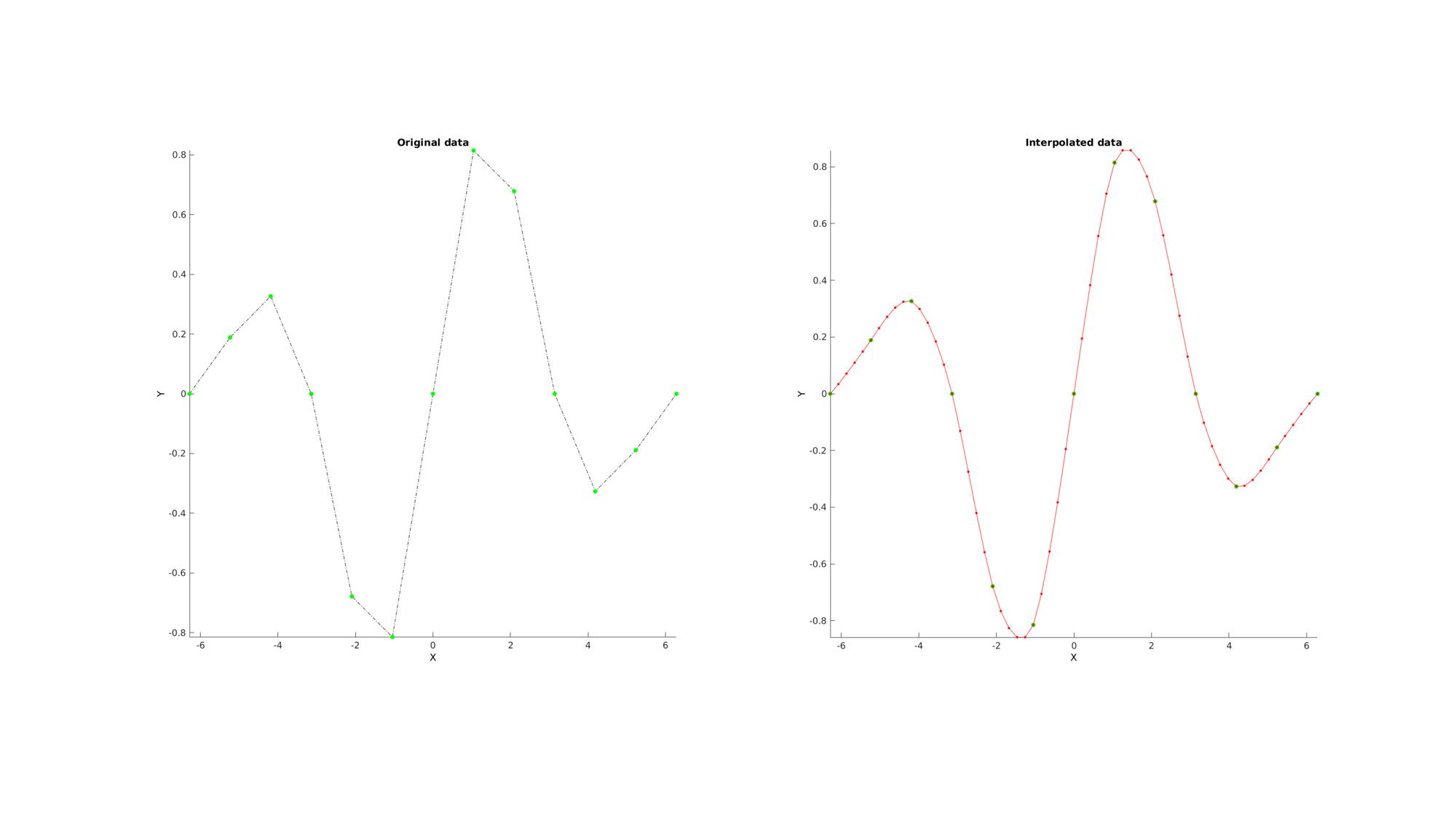
Example: 1D Interpolation

Below is an example for 1D curve interpolation

n=13;
x=linspace(-2*pi,2*pi,n);
y=exp( -0.5.*(x.^2./3.^2) ).*sin(x);

ni=n+4*(n-1);
xi=linspace(min(x(:)),max(x(:)),ni);
yi=biharmonicSplineInterpolation(x,y,xi);

Visualizing results

cFigure(figStruct);
subplot(1,2,1);
title('Original data','FontSize',fontSize);
xlabel('X','FontSize',fontSize); ylabel('Y','FontSize',fontSize); zlabel('Z','FontSize',fontSize)
hold on;
plot(x,y,'k-.');
plot(x,y,'g.','MarkerSize',markerSize1);
axis tight;  axis vis3d; grid off;  set(gca,'FontSize',fontSize);

subplot(1,2,2);
title('Interpolated data','FontSize',fontSize);
xlabel('X','FontSize',fontSize); ylabel('Y','FontSize',fontSize); zlabel('Z','FontSize',fontSize)
hold on;
plot(x,y,'g.','MarkerSize',markerSize1);
plot(xi,yi,'r.-','MarkerSize',markerSize1/2);
axis tight;  axis vis3d; grid off;  set(gca,'FontSize',fontSize);
drawnow;

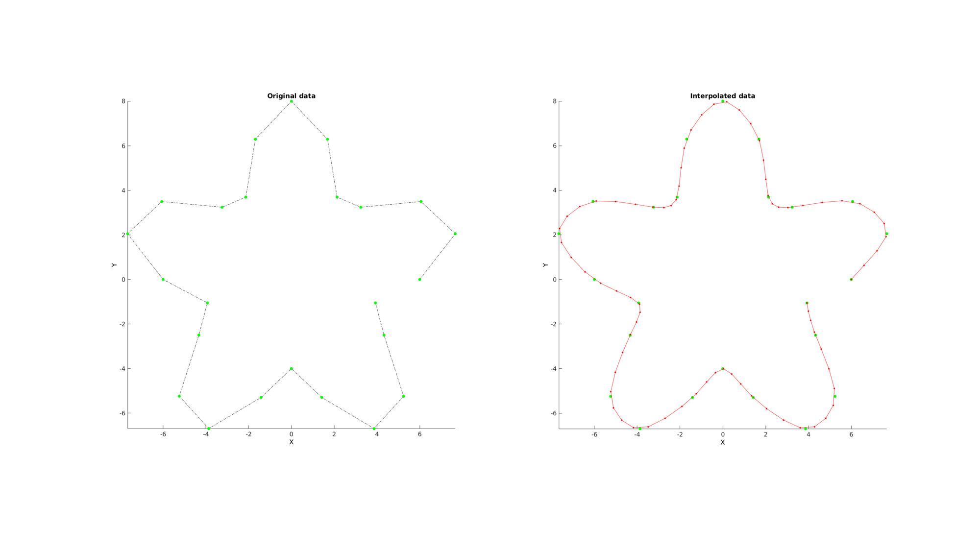
Example: Parametric curve interpolation

Below is an example for curve interpolation using a parametric representation

%Simulating a complex curve
n=25;
t=linspace(0,2*pi,n);
t=t(1:end-1);
r=6+2.*sin(5*t);
x=r.*cos(t);
y=r.*sin(t);

ni=n*3;
ti=linspace(min(t(:)),max(t(:)),ni);
xi=biharmonicSplineInterpolation(t,x,ti);
yi=biharmonicSplineInterpolation(t,y,ti);

Visualizing results

cFigure(figStruct);
subplot(1,2,1);
title('Original data','FontSize',fontSize);
xlabel('X','FontSize',fontSize); ylabel('Y','FontSize',fontSize); zlabel('Z','FontSize',fontSize)
hold on;
plot(x,y,'k-.');
plot(x,y,'g.','MarkerSize',markerSize1);
axis tight;  axis vis3d; grid off;  set(gca,'FontSize',fontSize);

subplot(1,2,2);
title('Interpolated data','FontSize',fontSize);
xlabel('X','FontSize',fontSize); ylabel('Y','FontSize',fontSize); zlabel('Z','FontSize',fontSize)
hold on;
plot(x,y,'g.','MarkerSize',markerSize1);
plot(xi,yi,'r.-','MarkerSize',markerSize1/2);
axis tight;  axis vis3d; grid off;  set(gca,'FontSize',fontSize);
drawnow;

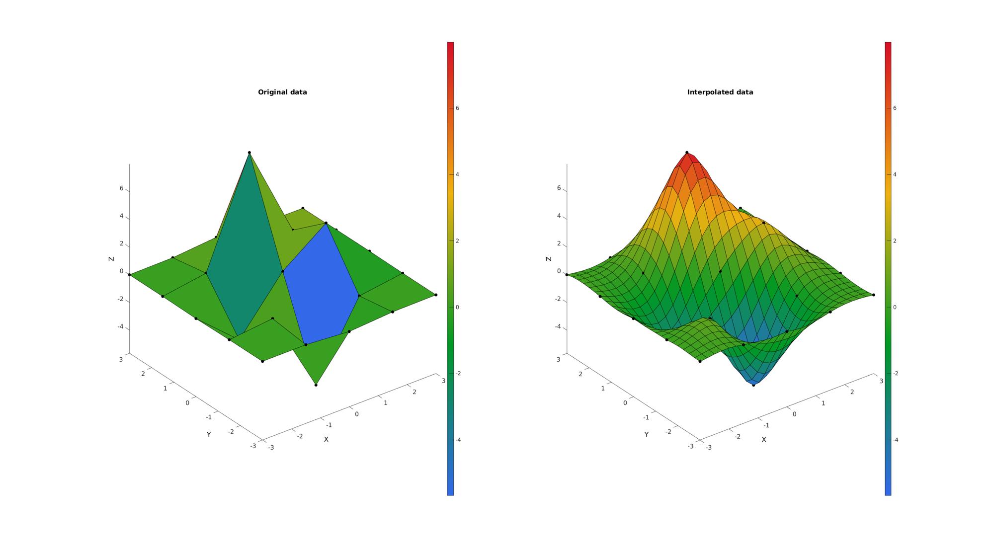
Example: 2D Interpolation

Below is an example for surface interpolation

n=5;
[X,Y,Z]=peaks(n);
[F,V,C]=surf2patch(X,Y,Z,Z);

XX=[X(:) Y(:)];

ni=25;
[XI,YI]=ndgrid(linspace(min(X(:)),max(X(:)),ni),linspace(min(Y(:)),max(Y(:)),ni));
XXI=[XI(:) YI(:)];
ZI=biharmonicSplineInterpolation(XX,Z,XXI);
ZI=reshape(ZI,size(XI));

[FI,VI,CI]=surf2patch(XI,YI,ZI,ZI);

Visualizing results

cFigure(figStruct);
subplot(1,2,1);
title('Original data','FontSize',fontSize);
xlabel('X','FontSize',fontSize); ylabel('Y','FontSize',fontSize); zlabel('Z','FontSize',fontSize)
hold on;
plotV(V,'k.','MarkerSize',markerSize1);
hs=patch('Faces',F,'Vertices',V,'EdgeColor','k', 'CData',C,'FaceColor','flat');
view(3); axis tight;  axis vis3d; grid off;  set(gca,'FontSize',fontSize);
colormap(cMap); colorbar;

subplot(1,2,2);
title('Interpolated data','FontSize',fontSize);
xlabel('X','FontSize',fontSize); ylabel('Y','FontSize',fontSize); zlabel('Z','FontSize',fontSize)
hold on;
plotV(V,'k.','MarkerSize',markerSize1);
hs=patch('Faces',FI,'Vertices',VI,'EdgeColor','k', 'CData',CI,'FaceColor','flat');
view(3); axis tight;  axis vis3d; grid off;  set(gca,'FontSize',fontSize);
colormap(cMap); colorbar;
drawnow;

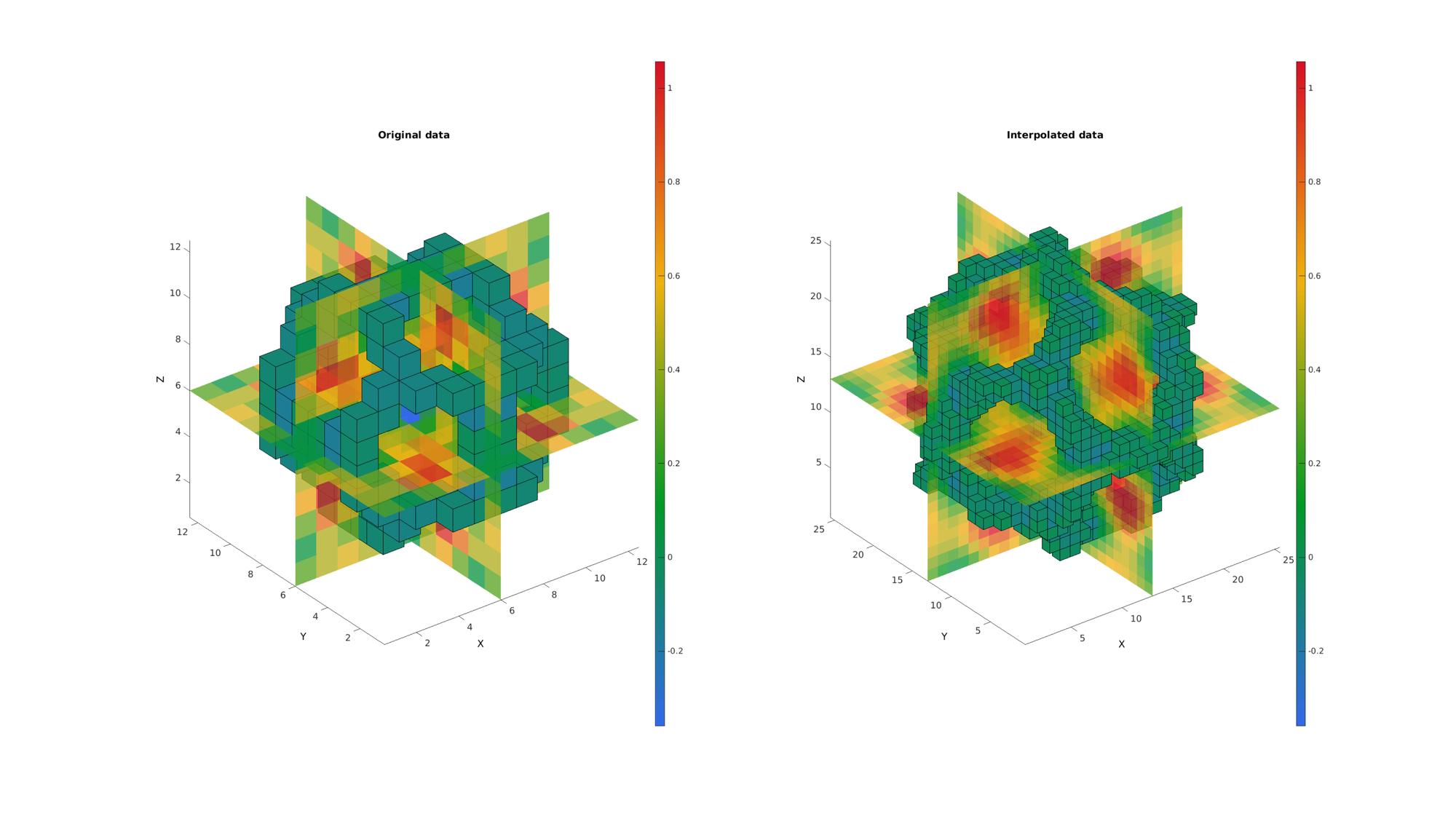
Example: 3D Interpolation

Below is an example for 3D (i.e. an image) interpolation

n=12;
[X,Y,Z]=meshgrid(linspace(-4.77,4.77,n));

phi=(1+sqrt(5))/2;
M=1/6*(2 - (cos(X + phi*Y) + cos(X - phi*Y) + cos(Y + phi*Z) + cos(Y - phi*Z) + cos(Z - phi*X) + cos(Z + phi*X)));

XX=[X(:) Y(:) Z(:)];

ni=25;
[XI,YI,ZI]=ndgrid(linspace(min(X(:)),max(X(:)),ni),linspace(min(Y(:)),max(Y(:)),ni),linspace(min(Z(:)),max(Z(:)),ni));
XXI=[XI(:) YI(:) ZI(:)];
MI=biharmonicSplineInterpolation(XX,M,XXI);
MI=reshape(MI,size(XI));

Visualizing results

cFigure(figStruct);
subplot(1,2,1);
title('Original data','FontSize',fontSize);
xlabel('X','FontSize',fontSize); ylabel('Y','FontSize',fontSize); zlabel('Z','FontSize',fontSize)
hold on;

% Setting up indices for I direction slices
S=round(size(M,1)./2); %Selection of middle slice
L_plot=false(size(M)); L_plot(S,:,:)=1;
IND=find(L_plot);
[F,V,C]=ind2patch(IND,M,'si'); %Creating patch data for y mid-voxel slices
hs=patch('Faces',F,'Vertices',V,'EdgeColor','none', 'CData',C,'FaceColor','flat','FaceAlpha',0.75);

% Setting up indices for J direction slices
S=round(size(M,2)./2); %Selection of middle slice
L_plot=false(size(M)); L_plot(:,S,:)=1;
IND=find(L_plot);
[F,V,C]=ind2patch(IND,M,'sj'); %Creating patch data for x mid-voxel slices
hs=patch('Faces',F,'Vertices',V,'EdgeColor','none', 'CData',C,'FaceColor','flat','FaceAlpha',0.75);

% Setting up indices for K direction slices
S=round(size(M,3)./2); %Selection of middle slice
L_plot=false(size(M)); L_plot(:,:,S)=1;
IND=find(L_plot);
[F,V,C]=ind2patch(IND,M,'sk'); %Creating patch data for z mid-voxel slices
hs=patch('Faces',F,'Vertices',V,'EdgeColor','none', 'CData',C,'FaceColor','flat','FaceAlpha',0.75);

% Setting up indices for voxels to plot
L_mask=M>-0.2 & M<0;
[F,V,C]=ind2patch(L_mask,M,'vb'); %Creating patch data for selection of high voxels

hs=patch('Faces',F,'Vertices',V,'EdgeColor','k', 'CData',C,'FaceColor','flat','FaceAlpha',1);

colormap(cMap); colorbar; caxis([min(M(:)) max(M(:))]);
view(3); axis tight;  axis vis3d; grid off;  set(gca,'FontSize',fontSize);

subplot(1,2,2);
title('Interpolated data','FontSize',fontSize);
xlabel('X','FontSize',fontSize); ylabel('Y','FontSize',fontSize); zlabel('Z','FontSize',fontSize)
hold on;

% Setting up indices for I direction slices
S=round(size(MI,1)./2); %Selection of middle slice
L_plot=false(size(MI)); L_plot(S,:,:)=1;
IND=find(L_plot);
[F,V,C]=ind2patch(IND,MI,'si'); %Creating patch data for y mid-voxel slices
hs=patch('Faces',F,'Vertices',V,'EdgeColor','none', 'CData',C,'FaceColor','flat','FaceAlpha',0.75);

% Setting up indices for J direction slices
S=round(size(MI,2)./2); %Selection of middle slice
L_plot=false(size(MI)); L_plot(:,S,:)=1;
IND=find(L_plot);
[F,V,C]=ind2patch(IND,MI,'sj'); %Creating patch data for x mid-voxel slices
hs=patch('Faces',F,'Vertices',V,'EdgeColor','none', 'CData',C,'FaceColor','flat','FaceAlpha',0.75);

% Setting up indices for K direction slices
S=round(size(MI,3)./2); %Selection of middle slice
L_plot=false(size(MI)); L_plot(:,:,S)=1;
IND=find(L_plot);
[F,V,C]=ind2patch(IND,MI,'sk'); %Creating patch data for z mid-voxel slices
hs=patch('Faces',F,'Vertices',V,'EdgeColor','none', 'CData',C,'FaceColor','flat','FaceAlpha',0.75);

% Setting up indices for voxels to plot
L_mask=MI>-0.2 & MI<0;
[F,V,C]=ind2patch(L_mask,MI,'vb'); %Creating patch data for selection of high voxels

hs=patch('Faces',F,'Vertices',V,'EdgeColor','k', 'CData',C,'FaceColor','flat','FaceAlpha',1);

colormap(cMap); colorbar; caxis([min(M(:)) max(M(:))]);
view(3); axis tight;  axis vis3d; grid off;  set(gca,'FontSize',fontSize);
drawnow;

GIBBON www.gibboncode.org

Kevin Mattheus Moerman, [email protected]

GIBBON footer text

License: https://github.com/gibbonCode/GIBBON/blob/master/LICENSE

GIBBON: The Geometry and Image-based Bioengineering add-On. A toolbox for image segmentation, image-based modeling, meshing, and finite element analysis.

Copyright (C) 2019 Kevin Mattheus Moerman

This program is free software: you can redistribute it and/or modify it under the terms of the GNU General Public License as published by the Free Software Foundation, either version 3 of the License, or (at your option) any later version.

This program is distributed in the hope that it will be useful, but WITHOUT ANY WARRANTY; without even the implied warranty of MERCHANTABILITY or FITNESS FOR A PARTICULAR PURPOSE. See the GNU General Public License for more details.

You should have received a copy of the GNU General Public License along with this program. If not, see http://www.gnu.org/licenses/.

Published with MATLAB® R2019a