adjacentdircount

Below is a demonstration of the features of the adjacentdircount function

Syntax
Description
Examples
Example: Using adjacentdircount to compute "connectivity"
Example: Use for 3D arrays
Example: Studying object line feature thickness

Syntax

[Lc]=adjacentdircount(L,n);

Description

The adjacentdircount function calculates the number of adjacent entries of an input logic array allong a specified direction.

Examples

clear; close all; clc;

Plot settings

fontSize=10;

Example: Using `adjacentdircount` to compute "connectivity"

The adjacentdircount function computes the number of adjacent elements in the input array that have the value 1. As such it computes a type of connectivity or "thickness" of structures in the logic arrays allong a certain dimension.

Lets consider the following array:

L=[0 1 1 0 0 1;...
   0 0 1 0 0 1;...
   1 0 0 1 1 1]; %A logic array or an array containing ones

Now view the output of the adjacentdircount function for n=1:

n=1; %Row direction (i.e. thickness orthogonal to rows)
[Lc]=adjacentdircount(L,n);
Lc

Lc =

     0     1     2     0     0     3
     0     0     2     0     0     3
     1     0     0     1     1     3

and similarly for for n=2:

n=2; %Column direction (i.e. thickness orthogonal to columns)
[Lc]=adjacentdircount(L,n);
Lc

Lc =

     0     2     2     0     0     1
     0     0     1     0     0     1
     1     0     0     3     3     3

Example: Use for 3D arrays

Create a 3D example array, here L is copied upside down into a second "slice" and again for the third slice.

L(:,:,2)=flipud(L);
L(:,:,3)=flipud(L(:,:,1));

n=3; %Slice direction (i.e. thickness orthogonal to slices)
[Lc]=adjacentdircount(L,n);
Lc

Lc(:,:,1) =

     0     1     1     0     0     3
     0     0     3     0     0     3
     1     0     0     1     1     3


Lc(:,:,2) =

     2     0     0     2     2     3
     0     0     3     0     0     3
     0     2     2     0     0     3


Lc(:,:,3) =

     2     0     0     2     2     3
     0     0     3     0     0     3
     0     2     2     0     0     3

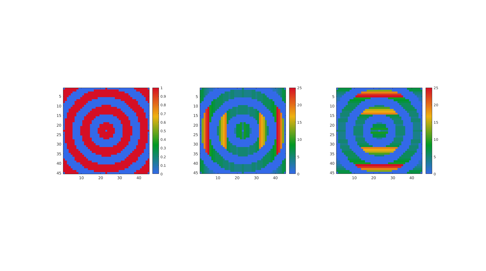
Example: Studying object line feature thickness

% Simulating a striped image in 3D
np=45;
[X,Y,Z]=meshgrid(linspace(-5*pi,5*pi,np));
R=sqrt(X.^2+Y.^2+Z.^2); %Radii
M=sin(R);

First consider the mid-slice for 2D analysis

midInd=round(size(M,3)/2);
m=M(:,:,midInd);

Convert to a logic array for thickness analysis

L=m>0;

Now use adjacentdircount to compute "connectivity" allong first and second dimensions

[Lc1]=adjacentdircount(L,1); %1st dim
[Lc2]=adjacentdircount(L,2); %1st dim

Plotting the results

hf=cFigure;
hold on;
subplot(1,3,1);
imagesc(L);
colormap gjet; colorbar;
axis equal; axis tight;
set(gca,'FontSize',fontSize);

subplot(1,3,2);
imagesc(Lc1);
colormap gjet; colorbar;
axis equal; axis tight;
set(gca,'FontSize',fontSize);

subplot(1,3,3);
imagesc(Lc2);
colormap gjet; colorbar;
axis equal; axis tight;
set(gca,'FontSize',fontSize);

drawnow;

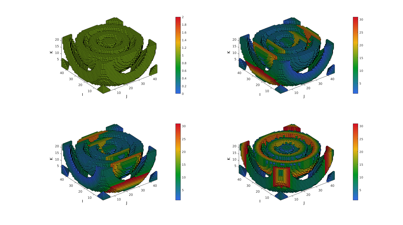
Now lets expand to 3D analysis

L=M>0;
[Lc1]=adjacentdircount(L,1); %1st dim
[Lc2]=adjacentdircount(L,2); %1st dim
[Lc3]=adjacentdircount(L,3); %1st dim

%Construct logic array setting voxels to display using |ind2patch| function
logicPatch=L; %Initialise as L
logicPatch(:,:,midInd:end)=0; %Crop off half to visualize interior

[F,V,C]=ind2patch(logicPatch,L,'vb');
[F1,V1,C1]=ind2patch(logicPatch,Lc1,'vb');
[F2,V2,C2]=ind2patch(logicPatch,Lc2,'vb');
[F3,V3,C3]=ind2patch(logicPatch,Lc3,'vb');

cFigure;
subplot(2,2,1);
xlabel('J');ylabel('I'); zlabel('K'); hold on;
patch('Faces',F,'Vertices',V,'FaceColor','flat','CData',C,'EdgeColor','k');
axis equal; view(3); axis tight; axis vis3d; grid off;
colormap gjet; colorbar;
set(gca,'FontSize',fontSize);

subplot(2,2,2);
xlabel('J');ylabel('I'); zlabel('K'); hold on;
patch('Faces',F1,'Vertices',V1,'FaceColor','flat','CData',C1,'EdgeColor','k');
axis equal; view(3); axis tight; axis vis3d; grid off;
colormap gjet; colorbar;
set(gca,'FontSize',fontSize);

subplot(2,2,3);
xlabel('J');ylabel('I'); zlabel('K'); hold on;
patch('Faces',F2,'Vertices',V2,'FaceColor','flat','CData',C2,'EdgeColor','k');
axis equal; view(3); axis tight; axis vis3d; grid off;
colormap gjet; colorbar;
set(gca,'FontSize',fontSize);

subplot(2,2,4);
xlabel('J');ylabel('I'); zlabel('K'); hold on;
patch('Faces',F3,'Vertices',V3,'FaceColor','flat','CData',C3,'EdgeColor','k');
axis equal; view(3); axis tight; axis vis3d; grid off;
colormap gjet; colorbar;
set(gca,'FontSize',fontSize);

drawnow;

GIBBON www.gibboncode.org

Kevin Mattheus Moerman, [email protected]

GIBBON footer text

License: https://github.com/gibbonCode/GIBBON/blob/master/LICENSE

GIBBON: The Geometry and Image-based Bioengineering add-On. A toolbox for image segmentation, image-based modeling, meshing, and finite element analysis.

This program is free software: you can redistribute it and/or modify it under the terms of the GNU General Public License as published by the Free Software Foundation, either version 3 of the License, or (at your option) any later version.

This program is distributed in the hope that it will be useful, but WITHOUT ANY WARRANTY; without even the implied warranty of MERCHANTABILITY or FITNESS FOR A PARTICULAR PURPOSE. See the GNU General Public License for more details.

You should have received a copy of the GNU General Public License along with this program. If not, see http://www.gnu.org/licenses/.