DEMO_febio_0076_actuator_donnan_equilibrium_swelling_01
Below is a demonstration for:
- Building geometry for a cube with hexahedral elements
- Defining the boundary conditions
- Coding the febio structure
- Running the model
- Importing and visualizing the displacement and stress results
Contents
Keywords
- febio_spec version 3.0
- febio, FEBio
- donnan equilibrium swelling
- hexahedral elements, hex8
- cube, box, rectangular
- static, solid
- displacement logfile
- stress logfile
clear; close all; clc;
Plot settings
fontSize=20;
faceAlpha1=0.8;
markerSize=40;
markerSize2=25;
lineWidth=3;
cMap=spectral(250); %colormap
Control parameters
% Path names
defaultFolder = fileparts(fileparts(mfilename('fullpath')));
savePath=fullfile(defaultFolder,'data','temp');

% Defining file names
febioFebFileNamePart='tempModel';
febioFebFileName=fullfile(savePath,[febioFebFileNamePart,'.feb']); %FEB file name
febioLogFileName=[febioFebFileNamePart,'.txt']; %FEBio log file name
febioLogFileName_disp=[febioFebFileNamePart,'_disp_out.txt']; %Log file name for exporting displacement
febioLogFileName_vol=[febioFebFileNamePart,'_vol_out.txt']; %Log file name for exporting stress
febioLogFileName_stress_prin=[febioFebFileNamePart,'_stress_prin_out.txt']; %Log file name for exporting principal stress

%Specifying dimensions and number of elements
sampleWidth=0.5; %Width
sampleThickness=1.5; %Thickness
sampleHeight=7; %Height
pointSpacings=0.25*ones(1,3); %Desired point spacing between nodes
numElementsWidth=round(sampleWidth/pointSpacings(1)); %Number of elemens in dir 1
numElementsThickness=round(sampleThickness/pointSpacings(2)); %Number of elemens in dir 2
numElementsHeight=round(sampleHeight/pointSpacings(3)); %Number of elemens in dir 3

%Material parameter set
E_youngs=1;
v_pois=0.3;

anisotropicOption=0;
if anisotropicOption==1
    ksi=[500 500 0.01];
    beta=[3 3 3];
end

bosm_ini=300;
bosm_diff_amp=200;
cF0=bosm_ini;

% FEA control settings
numTimeSteps=50; %Number of time steps desired
max_refs=25; %Max reforms
max_ups=0; %Set to zero to use full-Newton iterations
opt_iter=25; %Optimum number of iterations
max_retries=5; %Maximum number of retires
dtmin=(1/numTimeSteps)/100; %Minimum time step size
dtmax=1/numTimeSteps; %Maximum time step size

runMode='internal';
Creating model geometry and mesh
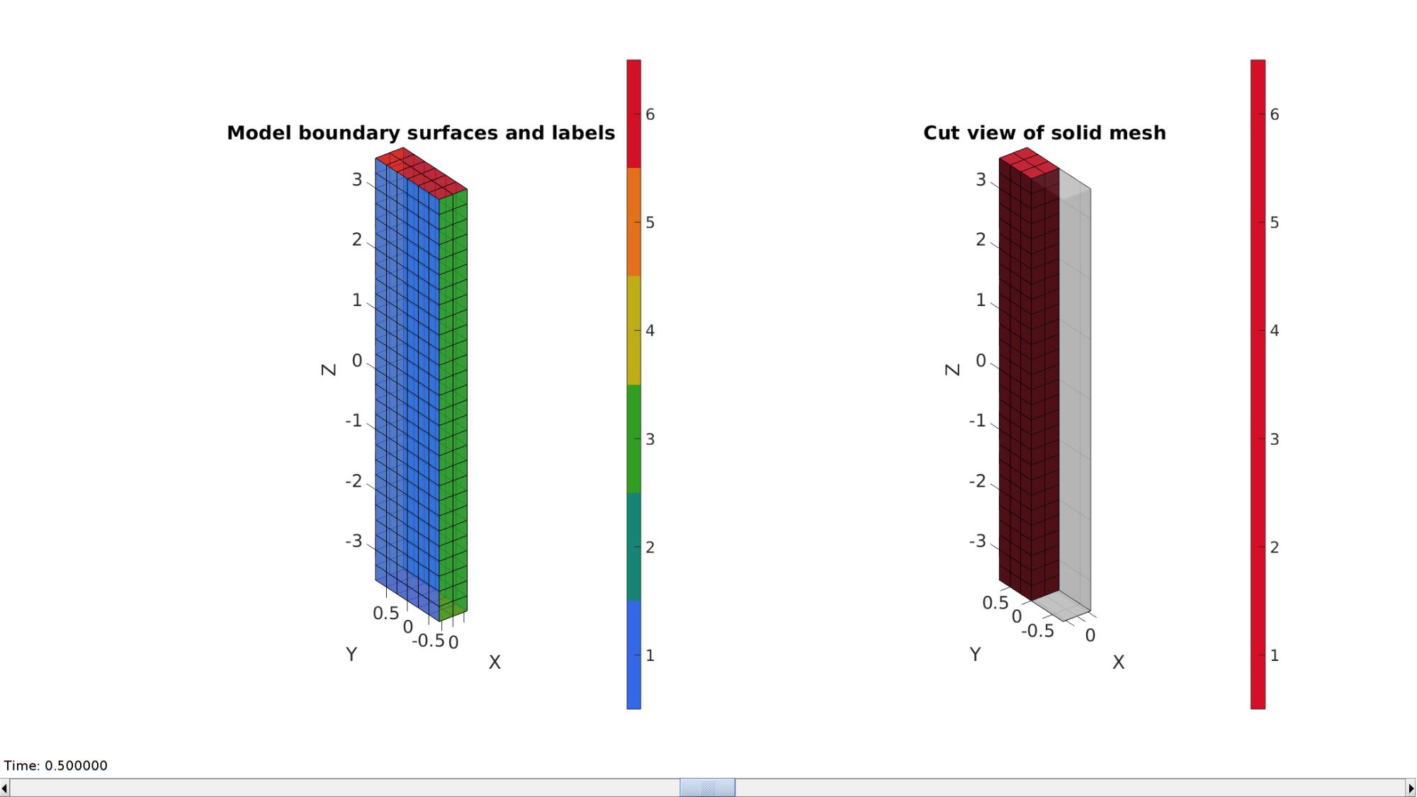
A box is created with tri-linear hexahedral (hex8) elements using the hexMeshBox function. The function offers the boundary faces with seperate labels for the top, bottom, left, right, front, and back sides. As such these can be used to define boundary conditions on the exterior.
% Create a box with hexahedral elements
cubeDimensions=[sampleWidth sampleThickness sampleHeight]; %Dimensions
cubeElementNumbers=[numElementsWidth numElementsThickness numElementsHeight]; %Number of elements
outputStructType=2; %A structure compatible with mesh view
[meshStruct]=hexMeshBox(cubeDimensions,cubeElementNumbers,outputStructType);

%Access elements, nodes, and faces from the structure
E=meshStruct.elements; %The elements
V=meshStruct.nodes; %The nodes (vertices)
Fb=meshStruct.facesBoundary; %The boundary faces
Cb=meshStruct.boundaryMarker; %The "colors" or labels for the boundary faces
elementMaterialIndices=ones(size(E,1),1); %Element material indices
VE=patchCentre(E,V);
logicSide=VE(:,1)<0;
E1=E(logicSide,:); %First set
E2=E(~logicSide,:); %Second set
E=[E1;E2]; %Reorder full set
Plotting model boundary surfaces and a cut view
hFig=cFigure;

subplot(1,2,1); hold on;
title('Model boundary surfaces and labels','FontSize',fontSize);
gpatch(Fb,V,Cb,'k',faceAlpha1);
colormap(gjet(6)); icolorbar;
axisGeom(gca,fontSize);

hs=subplot(1,2,2); hold on;
title('Cut view of solid mesh','FontSize',fontSize);
optionStruct.hFig=[hFig hs];
meshView(meshStruct,optionStruct);
axisGeom(gca,fontSize);

drawnow;
Defining the boundary conditions
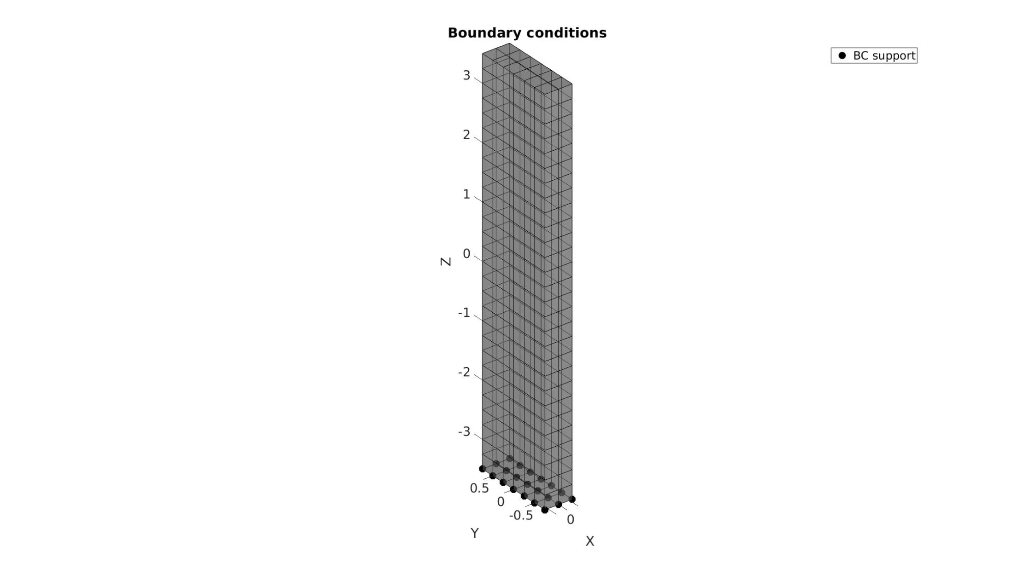
The visualization of the model boundary shows colors for each side of the cube. These labels can be used to define boundary conditions.
%Prescribed displacement nodes
bcSupportList=unique(Fb(Cb==5,:)); %Node set for selected face
Visualizing boundary conditions. Markers plotted on the semi-transparent model denote the nodes in the various boundary condition lists.
hf=cFigure;
title('Boundary conditions','FontSize',fontSize);
xlabel('X','FontSize',fontSize); ylabel('Y','FontSize',fontSize); zlabel('Z','FontSize',fontSize);
hold on;

gpatch(Fb,V,'kw','k',0.5);

hl(1)=plotV(V(bcSupportList,:),'k.','MarkerSize',markerSize);

legend(hl,{'BC support'});

axisGeom(gca,fontSize);
camlight headlight;
drawnow;
Defining the FEBio input structure
See also febioStructTemplate and febioStruct2xml and the FEBio user manual.
%Get a template with default settings
[febio_spec]=febioStructTemplate;

%febio_spec version
febio_spec.ATTR.version='4.0';

%Module section
febio_spec.Module.ATTR.type='biphasic';

%Control section
febio_spec.Control.analysis='STEADY-STATE';
febio_spec.Control.time_steps=numTimeSteps;
febio_spec.Control.step_size=1/numTimeSteps;
febio_spec.Control.solver.max_refs=max_refs;
febio_spec.Control.solver.qn_method.max_ups=max_ups;
febio_spec.Control.time_stepper.dtmin=dtmin;
% febio_spec.Control.time_stepper.dtmax=dtmax;
febio_spec.Control.time_stepper=rmfield(febio_spec.Control.time_stepper,'dtmax'); %Remove existing template dtmax definition
febio_spec.Control.time_stepper.dtmax.ATTR.lc=1; %Set load curve id for dtmax
febio_spec.Control.time_stepper.dtmax.VAL=1; %Set value
febio_spec.Control.time_stepper.max_retries=max_retries;
febio_spec.Control.time_stepper.opt_iter=opt_iter;

%Set globals/constants
febio_spec.Globals.Constants.R=8.314e-6;
febio_spec.Globals.Constants.T=310;

febio_spec.Output.plotfile.var{end+1}.ATTR.type='fluid pressure';
febio_spec.Output.plotfile.var{end+1}.ATTR.type='effective fluid pressure';

%Material section
materialName1='Material1';
febio_spec.Material.material{1}.ATTR.name=materialName1;
febio_spec.Material.material{1}.ATTR.type='solid mixture';
febio_spec.Material.material{1}.ATTR.id=1;
febio_spec.Material.material{1}.mat_axis.ATTR.type='vector';
febio_spec.Material.material{1}.mat_axis.a=[1 0 0];
febio_spec.Material.material{1}.mat_axis.d=[0 1 0];

febio_spec.Material.material{1}.solid{1}.ATTR.type='Donnan equilibrium';
febio_spec.Material.material{1}.solid{1}.phiw0=0.8;
febio_spec.Material.material{1}.solid{1}.cF0.ATTR.lc=2;
febio_spec.Material.material{1}.solid{1}.cF0.VAL=1;
febio_spec.Material.material{1}.solid{1}.bosm.ATTR.lc=3;
febio_spec.Material.material{1}.solid{1}.bosm.VAL=1;

febio_spec.Material.material{1}.solid{2}.ATTR.type='neo-Hookean';
febio_spec.Material.material{1}.solid{2}.E=1;
febio_spec.Material.material{1}.solid{2}.v=0.3;

if anisotropicOption==1
    febio_spec.Material.material{1}.solid{3}.ATTR.type='ellipsoidal fiber distribution';
    febio_spec.Material.material{1}.solid{3}.ksi=ksi;
    febio_spec.Material.material{1}.solid{3}.beta=beta;
end

materialName2='Material2';
febio_spec.Material.material{2}.ATTR.name=materialName2;
febio_spec.Material.material{2}.ATTR.type='solid mixture';
febio_spec.Material.material{2}.ATTR.id=2;
febio_spec.Material.material{1}.mat_axis.ATTR.type='vector';
febio_spec.Material.material{1}.mat_axis.a=[1 0 0];
febio_spec.Material.material{1}.mat_axis.d=[0 1 0];

febio_spec.Material.material{2}.solid{1}.ATTR.type='Donnan equilibrium';
febio_spec.Material.material{2}.solid{1}.phiw0=0.8;
febio_spec.Material.material{2}.solid{1}.cF0.ATTR.lc=2;
febio_spec.Material.material{2}.solid{1}.cF0.VAL=1;
febio_spec.Material.material{2}.solid{1}.bosm.ATTR.lc=4;
febio_spec.Material.material{2}.solid{1}.bosm.VAL=1;

febio_spec.Material.material{2}.solid{2}.ATTR.type='neo-Hookean';
febio_spec.Material.material{2}.solid{2}.E=E_youngs;
febio_spec.Material.material{2}.solid{2}.v=v_pois;

if anisotropicOption==1
    febio_spec.Material.material{2}.solid{3}.ATTR.type='ellipsoidal fiber distribution';
    febio_spec.Material.material{2}.solid{3}.ksi=ksi;
    febio_spec.Material.material{2}.solid{3}.beta=beta;
end

% Mesh section
% -> Nodes
febio_spec.Mesh.Nodes{1}.ATTR.name='Object1'; %The node set name
febio_spec.Mesh.Nodes{1}.node.ATTR.id=(1:size(V,1))'; %The node id's
febio_spec.Mesh.Nodes{1}.node.VAL=V; %The nodel coordinates

% -> Elements
partName1='Part1';
febio_spec.Mesh.Elements{1}.ATTR.name=partName1; %Name of this part
febio_spec.Mesh.Elements{1}.ATTR.type='hex8'; %Element type
febio_spec.Mesh.Elements{1}.elem.ATTR.id=(1:1:size(E1,1))'; %Element id's
febio_spec.Mesh.Elements{1}.elem.VAL=E1; %The element matrix

partName2='Part2';
febio_spec.Mesh.Elements{2}.ATTR.name=partName2; %Name of this part
febio_spec.Mesh.Elements{2}.ATTR.type='hex8'; %Element type
febio_spec.Mesh.Elements{2}.elem.ATTR.id=size(E1,1)+(1:1:size(E2,1))'; %Element id's
febio_spec.Mesh.Elements{2}.elem.VAL=E2; %The element matrix

% -> NodeSets
nodeSetName1='bcSupportList';

febio_spec.Mesh.NodeSet{1}.ATTR.name=nodeSetName1;
febio_spec.Mesh.NodeSet{1}.VAL=mrow(bcSupportList);

%MeshDomains section
febio_spec.MeshDomains.SolidDomain{1}.ATTR.name=partName1;
febio_spec.MeshDomains.SolidDomain{1}.ATTR.mat=materialName1;

febio_spec.MeshDomains.SolidDomain{2}.ATTR.name=partName2;
febio_spec.MeshDomains.SolidDomain{2}.ATTR.mat=materialName2;

%Boundary condition section
% -> Fix boundary conditions
febio_spec.Boundary.bc{1}.ATTR.name='zero_displacement_x';
febio_spec.Boundary.bc{1}.ATTR.type='zero displacement';
febio_spec.Boundary.bc{1}.ATTR.node_set=nodeSetName1;
febio_spec.Boundary.bc{1}.x_dof=1;
febio_spec.Boundary.bc{1}.y_dof=1;
febio_spec.Boundary.bc{1}.z_dof=1;

%LoadData section
% -> load_controller
febio_spec.LoadData.load_controller{1}.ATTR.name='LC_1';
febio_spec.LoadData.load_controller{1}.ATTR.id=1;
febio_spec.LoadData.load_controller{1}.ATTR.type='loadcurve';
febio_spec.LoadData.load_controller{1}.interpolate='STEP';
febio_spec.LoadData.load_controller{1}.points.pt.VAL=[0 dtmax; 0.2 dtmax; 0.4 dtmax; 0.6 dtmax; 0.8 dtmax; 1 dtmax];

febio_spec.LoadData.load_controller{2}.ATTR.name='LC_2';
febio_spec.LoadData.load_controller{2}.ATTR.id=2;
febio_spec.LoadData.load_controller{2}.ATTR.type='loadcurve';
febio_spec.LoadData.load_controller{2}.interpolate='LINEAR';
febio_spec.LoadData.load_controller{2}.points.pt.VAL=[0 0; 0.2 cF0; 1 cF0];

febio_spec.LoadData.load_controller{3}.ATTR.name='LC_3';
febio_spec.LoadData.load_controller{3}.ATTR.id=3;
febio_spec.LoadData.load_controller{3}.ATTR.type='loadcurve';
febio_spec.LoadData.load_controller{3}.interpolate='LINEAR';
febio_spec.LoadData.load_controller{3}.points.pt.VAL=[0 bosm_ini; 0.2 bosm_ini; 0.4 bosm_ini+bosm_diff_amp; 0.6 bosm_ini; 0.8 bosm_ini-bosm_diff_amp; 1 bosm_ini];

febio_spec.LoadData.load_controller{4}.ATTR.name='LC_4';
febio_spec.LoadData.load_controller{4}.ATTR.id=4;
febio_spec.LoadData.load_controller{4}.ATTR.type='loadcurve';
febio_spec.LoadData.load_controller{4}.interpolate='LINEAR';
febio_spec.LoadData.load_controller{4}.points.pt.VAL=[0 bosm_ini; 0.2 bosm_ini; 0.4 bosm_ini-bosm_diff_amp; 0.6 bosm_ini; 0.8 bosm_ini+bosm_diff_amp; 1 bosm_ini];

%Output section
% -> log file
febio_spec.Output.logfile.ATTR.file=febioLogFileName;
febio_spec.Output.logfile.node_data{1}.ATTR.file=febioLogFileName_disp;
febio_spec.Output.logfile.node_data{1}.ATTR.data='ux;uy;uz';
febio_spec.Output.logfile.node_data{1}.ATTR.delim=',';

febio_spec.Output.logfile.element_data{1}.ATTR.file=febioLogFileName_vol;
febio_spec.Output.logfile.element_data{1}.ATTR.data='J';
febio_spec.Output.logfile.element_data{1}.ATTR.delim=',';

febio_spec.Output.logfile.element_data{2}.ATTR.file=febioLogFileName_stress_prin;
febio_spec.Output.logfile.element_data{2}.ATTR.data='s1;s2;s3';
febio_spec.Output.logfile.element_data{2}.ATTR.delim=',';

% Plotfile section
febio_spec.Output.plotfile.compression=0;
Quick viewing of the FEBio input file structure
The febView function can be used to view the xml structure in a MATLAB figure window.
febView(febio_spec); %Viewing the febio file
Exporting the FEBio input file
Exporting the febio_spec structure to an FEBio input file is done using the febioStruct2xml function.
febioStruct2xml(febio_spec,febioFebFileName); %Exporting to file and domNode
%system(['gedit ',febioFebFileName,' &']);
Running the FEBio analysis
To run the analysis defined by the created FEBio input file the runMonitorFEBio function is used. The input for this function is a structure defining job settings e.g. the FEBio input file name. The optional output runFlag informs the user if the analysis was run succesfully.
febioAnalysis.run_filename=febioFebFileName; %The input file name
febioAnalysis.run_logname=febioLogFileName; %The name for the log file
febioAnalysis.disp_on=1; %Display information on the command window
febioAnalysis.runMode=runMode;
febioAnalysis.maxLogCheckTime=10; %Max log file checking time

[runFlag]=runMonitorFEBio(febioAnalysis);%START FEBio NOW!!!!!!!!
%%%%%%%%%%%%%%%%%%%%%%%%%%%%%%%%%%%%%%%%%%%%%%%%%%%%%%%%%%%%%%%%%%%%%%%%%%%
--------> RUNNING/MONITORING FEBIO JOB <-------- 01-May-2023 10:57:52
FEBio path: /home/kevin/FEBioStudio/bin/febio4
# Attempt removal of existing log files 01-May-2023 10:57:52
* Removal succesful 01-May-2023 10:57:52
# Attempt removal of existing .xplt files 01-May-2023 10:57:52
* Removal succesful 01-May-2023 10:57:52
# Starting FEBio... 01-May-2023 10:57:52
Max. total analysis time is: Inf s
===========================================================================
________ _________ _______ __ _________
| |\ | |\ | \\ | |\ / \\
| ____|| | ____|| | __ || |__|| | ___ ||
| |\___\| | |\___\| | |\_| || \_\| | // \ ||
| ||__ | ||__ | ||_| || | |\ | || | ||
| |\ | |\ | \\ | || | || | ||
| ___|| | ___|| | ___ || | || | || | ||
| |\__\| | |\__\| | |\__| || | || | || | ||
| || | ||___ | ||__| || | || | \\__/ ||
| || | |\ | || | || | ||
|___|| |________|| |_________// |__|| \_________//
F I N I T E E L E M E N T S F O R B I O M E C H A N I C S
version 4.1.0
FEBio is a registered trademark.
copyright (c) 2006-2023 - All rights reserved
===========================================================================
Default linear solver: pardiso
Success loading plugin libFEBioChem.so (version 1.0.0)
Success loading plugin libFEBioHeat.so (version 2.0.0)
Reading file /home/kevin/GIBBON/data/temp/tempModel.feb ...SUCCESS!
*************************************************************************
* WARNING *
* dtmax is ignored when specifying must points. *
*************************************************************************
Data Record #1
===========================================================================
Step = 0
Time = 0
Data = ux;uy;uz
File = /home/kevin/GIBBON/data/temp/tempModel_disp_out.txt
Data Record #2
===========================================================================
Step = 0
Time = 0
Data = J
File = /home/kevin/GIBBON/data/temp/tempModel_vol_out.txt
Data Record #3
===========================================================================
Step = 0
Time = 0
Data = s1;s2;s3
File = /home/kevin/GIBBON/data/temp/tempModel_stress_prin_out.txt
]0;(0%) tempModel.feb - FEBio 4.1.0 ]0;(0%) tempModel.feb - FEBio 4.1.0
*************************************************************************
* Selecting linear solver pardiso *
*************************************************************************
===== beginning time step 1 : 0.02 =====
Reforming stiffness matrix: reformation #1
===== reforming stiffness matrix:
Nr of equations ........................... : 1764
Nr of nonzeroes in stiffness matrix ....... : 49959
1
Nonlinear solution status: time= 0.02
stiffness updates = 0
right hand side evaluations = 2
stiffness matrix reformations = 1
step from line search = 1.000000
convergence norms : INITIAL CURRENT REQUIRED
residual 2.264168e-05 7.725090e-11 0.000000e+00
energy 9.213128e-05 1.690368e-07 9.213128e-07
displacement 2.542020e-02 2.542020e-02 2.542020e-08
Reforming stiffness matrix: reformation #2
2
Nonlinear solution status: time= 0.02
stiffness updates = 0
right hand side evaluations = 3
stiffness matrix reformations = 2
step from line search = 1.000000
convergence norms : INITIAL CURRENT REQUIRED
residual 2.264168e-05 9.713161e-22 0.000000e+00
energy 9.213128e-05 1.127856e-15 9.213128e-07
displacement 2.542020e-02 9.743538e-08 2.551975e-08
*************************************************************************
* WARNING *
* No force acting on the system. *
*************************************************************************
convergence summary
number of iterations : 2
number of reformations : 2
------- converged at time : 0.02
Data Record #1
===========================================================================
Step = 1
Time = 0.02
Data = ux;uy;uz
File = /home/kevin/GIBBON/data/temp/tempModel_disp_out.txt
Data Record #2
===========================================================================
Step = 1
Time = 0.02
Data = J
File = /home/kevin/GIBBON/data/temp/tempModel_vol_out.txt
Data Record #3
===========================================================================
Step = 1
Time = 0.02
Data = s1;s2;s3
File = /home/kevin/GIBBON/data/temp/tempModel_stress_prin_out.txt
]0;(2%) tempModel.feb - FEBio 4.1.0
===== beginning time step 2 : 0.04 =====
Reforming stiffness matrix: reformation #1
1
Nonlinear solution status: time= 0.04
stiffness updates = 0
right hand side evaluations = 2
stiffness matrix reformations = 1
step from line search = 1.000000
convergence norms : INITIAL CURRENT REQUIRED
residual 1.965375e-04 6.058365e-09 0.000000e+00
energy 7.836947e-04 4.323379e-06 7.836947e-06
displacement 2.118920e-01 2.118920e-01 2.118920e-07
Reforming stiffness matrix: reformation #2
2
Nonlinear solution status: time= 0.04
stiffness updates = 0
right hand side evaluations = 3
stiffness matrix reformations = 2
step from line search = 1.000000
convergence norms : INITIAL CURRENT REQUIRED
residual 1.965375e-04 6.246037e-18 0.000000e+00
energy 7.836947e-04 7.902566e-13 7.836947e-06
displacement 2.118920e-01 7.420086e-06 2.144053e-07
Reforming stiffness matrix: reformation #3
3
Nonlinear solution status: time= 0.04
stiffness updates = 0
right hand side evaluations = 4
stiffness matrix reformations = 3
step from line search = 1.000000
convergence norms : INITIAL CURRENT REQUIRED
residual 1.965375e-04 2.209069e-30 0.000000e+00
energy 7.836947e-04 2.018860e-25 7.836947e-06
displacement 2.118920e-01 9.227832e-15 2.144054e-07
convergence summary
number of iterations : 3
number of reformations : 3
------- converged at time : 0.04
Data Record #1
===========================================================================
Step = 2
Time = 0.04
Data = ux;uy;uz
File = /home/kevin/GIBBON/data/temp/tempModel_disp_out.txt
Data Record #2
===========================================================================
Step = 2
Time = 0.04
Data = J
File = /home/kevin/GIBBON/data/temp/tempModel_vol_out.txt
Data Record #3
===========================================================================
Step = 2
Time = 0.04
Data = s1;s2;s3
File = /home/kevin/GIBBON/data/temp/tempModel_stress_prin_out.txt
]0;(4%) tempModel.feb - FEBio 4.1.0
===== beginning time step 3 : 0.06 =====
Reforming stiffness matrix: reformation #1
1
Nonlinear solution status: time= 0.06
stiffness updates = 0
right hand side evaluations = 2
stiffness matrix reformations = 1
step from line search = 1.000000
convergence norms : INITIAL CURRENT REQUIRED
residual 5.018667e-04 4.145893e-08 0.000000e+00
energy 1.951525e-03 1.763242e-05 1.951525e-05
displacement 5.146962e-01 5.146962e-01 5.146962e-07
Reforming stiffness matrix: reformation #2
2
Nonlinear solution status: time= 0.06
stiffness updates = 0
right hand side evaluations = 3
stiffness matrix reformations = 2
step from line search = 1.000000
convergence norms : INITIAL CURRENT REQUIRED
residual 5.018667e-04 3.078010e-16 0.000000e+00
energy 1.951525e-03 1.424457e-11 1.951525e-05
displacement 5.146962e-01 4.880088e-05 5.247614e-07
Reforming stiffness matrix: reformation #3
3
Nonlinear solution status: time= 0.06
stiffness updates = 0
right hand side evaluations = 4
stiffness matrix reformations = 3
step from line search = 1.000000
convergence norms : INITIAL CURRENT REQUIRED
residual 5.018667e-04 2.180053e-30 0.000000e+00
energy 1.951525e-03 9.422475e-24 1.951525e-05
displacement 5.146962e-01 4.305748e-13 5.247624e-07
convergence summary
number of iterations : 3
number of reformations : 3
------- converged at time : 0.06
Data Record #1
===========================================================================
Step = 3
Time = 0.06
Data = ux;uy;uz
File = /home/kevin/GIBBON/data/temp/tempModel_disp_out.txt
Data Record #2
===========================================================================
Step = 3
Time = 0.06
Data = J
File = /home/kevin/GIBBON/data/temp/tempModel_vol_out.txt
Data Record #3
===========================================================================
Step = 3
Time = 0.06
Data = s1;s2;s3
File = /home/kevin/GIBBON/data/temp/tempModel_stress_prin_out.txt
]0;(6%) tempModel.feb - FEBio 4.1.0
===== beginning time step 4 : 0.08 =====
Reforming stiffness matrix: reformation #1
1
Nonlinear solution status: time= 0.08
stiffness updates = 0
right hand side evaluations = 2
stiffness matrix reformations = 1
step from line search = 1.000000
convergence norms : INITIAL CURRENT REQUIRED
residual 8.707252e-04 1.295497e-07 0.000000e+00
energy 3.297897e-03 4.000721e-05 3.297897e-05
displacement 8.475664e-01 8.475664e-01 8.475664e-07
Reforming stiffness matrix: reformation #2
2
Nonlinear solution status: time= 0.08
stiffness updates = 0
right hand side evaluations = 3
stiffness matrix reformations = 2
step from line search = 1.000000
convergence norms : INITIAL CURRENT REQUIRED
residual 8.707252e-04 3.130553e-15 0.000000e+00
energy 3.297897e-03 7.867457e-11 3.297897e-05
displacement 8.475664e-01 1.461169e-04 8.699549e-07
Reforming stiffness matrix: reformation #3
3
Nonlinear solution status: time= 0.08
stiffness updates = 0
right hand side evaluations = 4
stiffness matrix reformations = 3
step from line search = 1.000000
convergence norms : INITIAL CURRENT REQUIRED
residual 8.707252e-04 4.727713e-30 0.000000e+00
energy 3.297897e-03 3.464819e-22 3.297897e-05
displacement 8.475664e-01 4.144477e-12 8.699587e-07
convergence summary
number of iterations : 3
number of reformations : 3
------- converged at time : 0.08
Data Record #1
===========================================================================
Step = 4
Time = 0.08
Data = ux;uy;uz
File = /home/kevin/GIBBON/data/temp/tempModel_disp_out.txt
Data Record #2
===========================================================================
Step = 4
Time = 0.08
Data = J
File = /home/kevin/GIBBON/data/temp/tempModel_vol_out.txt
Data Record #3
===========================================================================
Step = 4
Time = 0.08
Data = s1;s2;s3
File = /home/kevin/GIBBON/data/temp/tempModel_stress_prin_out.txt
]0;(8%) tempModel.feb - FEBio 4.1.0
===== beginning time step 5 : 0.1 =====
Reforming stiffness matrix: reformation #1
1
Nonlinear solution status: time= 0.1
stiffness updates = 0
right hand side evaluations = 2
stiffness matrix reformations = 1
step from line search = 1.000000
convergence norms : INITIAL CURRENT REQUIRED
residual 1.241383e-03 2.684530e-07 0.000000e+00
energy 4.586819e-03 6.711030e-05 4.586819e-05
displacement 1.150510e+00 1.150510e+00 1.150510e-06
Reforming stiffness matrix: reformation #2
2
Nonlinear solution status: time= 0.1
stiffness updates = 0
right hand side evaluations = 3
stiffness matrix reformations = 2
step from line search = 1.000000
convergence norms : INITIAL CURRENT REQUIRED
residual 1.241383e-03 1.376495e-14 0.000000e+00
energy 4.586819e-03 2.327924e-10 4.586819e-05
displacement 1.150510e+00 2.906769e-04 1.187353e-06
Reforming stiffness matrix: reformation #3
3
Nonlinear solution status: time= 0.1
stiffness updates = 0
right hand side evaluations = 4
stiffness matrix reformations = 3
step from line search = 1.000000
convergence norms : INITIAL CURRENT REQUIRED
residual 1.241383e-03 4.485186e-29 0.000000e+00
energy 4.586819e-03 3.059530e-21 4.586819e-05
displacement 1.150510e+00 1.733813e-11 1.187362e-06
convergence summary
number of iterations : 3
number of reformations : 3
------- converged at time : 0.1
Data Record #1
===========================================================================
Step = 5
Time = 0.1
Data = ux;uy;uz
File = /home/kevin/GIBBON/data/temp/tempModel_disp_out.txt
Data Record #2
===========================================================================
Step = 5
Time = 0.1
Data = J
File = /home/kevin/GIBBON/data/temp/tempModel_vol_out.txt
Data Record #3
===========================================================================
Step = 5
Time = 0.1
Data = s1;s2;s3
File = /home/kevin/GIBBON/data/temp/tempModel_stress_prin_out.txt
]0;(10%) tempModel.feb - FEBio 4.1.0
===== beginning time step 6 : 0.12 =====
Reforming stiffness matrix: reformation #1
1
Nonlinear solution status: time= 0.12
stiffness updates = 0
right hand side evaluations = 2
stiffness matrix reformations = 1
step from line search = 1.000000
convergence norms : INITIAL CURRENT REQUIRED
residual 1.574552e-03 4.328481e-07 0.000000e+00
energy 5.692842e-03 9.394068e-05 5.692842e-05
displacement 1.397756e+00 1.397756e+00 1.397756e-06
Reforming stiffness matrix: reformation #2
2
Nonlinear solution status: time= 0.12
stiffness updates = 0
right hand side evaluations = 3
stiffness matrix reformations = 2
step from line search = 1.000000
convergence norms : INITIAL CURRENT REQUIRED
residual 1.574552e-03 3.603251e-14 0.000000e+00
energy 5.692842e-03 4.697108e-10 5.692842e-05
displacement 1.397756e+00 4.519107e-04 1.448443e-06
Reforming stiffness matrix: reformation #3
3
Nonlinear solution status: time= 0.12
stiffness updates = 0
right hand side evaluations = 4
stiffness matrix reformations = 3
step from line search = 1.000000
convergence norms : INITIAL CURRENT REQUIRED
residual 1.574552e-03 2.889991e-28 0.000000e+00
energy 5.692842e-03 1.263392e-20 5.692842e-05
displacement 1.397756e+00 4.349305e-11 1.448459e-06
convergence summary
number of iterations : 3
number of reformations : 3
------- converged at time : 0.12
Data Record #1
===========================================================================
Step = 6
Time = 0.12
Data = ux;uy;uz
File = /home/kevin/GIBBON/data/temp/tempModel_disp_out.txt
Data Record #2
===========================================================================
Step = 6
Time = 0.12
Data = J
File = /home/kevin/GIBBON/data/temp/tempModel_vol_out.txt
Data Record #3
===========================================================================
Step = 6
Time = 0.12
Data = s1;s2;s3
File = /home/kevin/GIBBON/data/temp/tempModel_stress_prin_out.txt
]0;(12%) tempModel.feb - FEBio 4.1.0
===== beginning time step 7 : 0.14 =====
Reforming stiffness matrix: reformation #1
1
Nonlinear solution status: time= 0.14
stiffness updates = 0
right hand side evaluations = 2
stiffness matrix reformations = 1
step from line search = 1.000000
convergence norms : INITIAL CURRENT REQUIRED
residual 1.852879e-03 5.929056e-07 0.000000e+00
energy 6.578255e-03 1.171447e-04 6.578255e-05
displacement 1.586383e+00 1.586383e+00 1.586383e-06
Reforming stiffness matrix: reformation #2
2
Nonlinear solution status: time= 0.14
stiffness updates = 0
right hand side evaluations = 3
stiffness matrix reformations = 2
step from line search = 1.000000
convergence norms : INITIAL CURRENT REQUIRED
residual 1.852879e-03 6.715844e-14 0.000000e+00
energy 6.578255e-03 7.389012e-10 6.578255e-05
displacement 1.586383e+00 5.999856e-04 1.648650e-06
Reforming stiffness matrix: reformation #3
3
Nonlinear solution status: time= 0.14
stiffness updates = 0
right hand side evaluations = 4
stiffness matrix reformations = 3
step from line search = 1.000000
convergence norms : INITIAL CURRENT REQUIRED
residual 1.852879e-03 9.701031e-28 0.000000e+00
energy 6.578255e-03 3.119525e-20 6.578255e-05
displacement 1.586383e+00 7.823567e-11 1.648672e-06
convergence summary
number of iterations : 3
number of reformations : 3
------- converged at time : 0.14
Data Record #1
===========================================================================
Step = 7
Time = 0.14
Data = ux;uy;uz
File = /home/kevin/GIBBON/data/temp/tempModel_disp_out.txt
Data Record #2
===========================================================================
Step = 7
Time = 0.14
Data = J
File = /home/kevin/GIBBON/data/temp/tempModel_vol_out.txt
Data Record #3
===========================================================================
Step = 7
Time = 0.14
Data = s1;s2;s3
File = /home/kevin/GIBBON/data/temp/tempModel_stress_prin_out.txt
]0;(14%) tempModel.feb - FEBio 4.1.0
===== beginning time step 8 : 0.16 =====
Reforming stiffness matrix: reformation #1
1
Nonlinear solution status: time= 0.16
stiffness updates = 0
right hand side evaluations = 2
stiffness matrix reformations = 1
step from line search = 1.000000
convergence norms : INITIAL CURRENT REQUIRED
residual 2.073596e-03 7.279360e-07 0.000000e+00
energy 7.253793e-03 1.353234e-04 7.253793e-05
displacement 1.723799e+00 1.723799e+00 1.723799e-06
Reforming stiffness matrix: reformation #2
2
Nonlinear solution status: time= 0.16
stiffness updates = 0
right hand side evaluations = 3
stiffness matrix reformations = 2
step from line search = 1.000000
convergence norms : INITIAL CURRENT REQUIRED
residual 2.073596e-03 9.957721e-14 0.000000e+00
energy 7.253793e-03 9.839759e-10 7.253793e-05
displacement 1.723799e+00 7.176816e-04 1.794821e-06
Reforming stiffness matrix: reformation #3
3
Nonlinear solution status: time= 0.16
stiffness updates = 0
right hand side evaluations = 4
stiffness matrix reformations = 3
step from line search = 1.000000
convergence norms : INITIAL CURRENT REQUIRED
residual 2.073596e-03 2.075785e-27 0.000000e+00
energy 7.253793e-03 5.482604e-20 7.253793e-05
displacement 1.723799e+00 1.126605e-10 1.794850e-06
convergence summary
number of iterations : 3
number of reformations : 3
------- converged at time : 0.16
Data Record #1
===========================================================================
Step = 8
Time = 0.16
Data = ux;uy;uz
File = /home/kevin/GIBBON/data/temp/tempModel_disp_out.txt
Data Record #2
===========================================================================
Step = 8
Time = 0.16
Data = J
File = /home/kevin/GIBBON/data/temp/tempModel_vol_out.txt
Data Record #3
===========================================================================
Step = 8
Time = 0.16
Data = s1;s2;s3
File = /home/kevin/GIBBON/data/temp/tempModel_stress_prin_out.txt
]0;(16%) tempModel.feb - FEBio 4.1.0
===== beginning time step 9 : 0.18 =====
Reforming stiffness matrix: reformation #1
1
Nonlinear solution status: time= 0.18
stiffness updates = 0
right hand side evaluations = 2
stiffness matrix reformations = 1
step from line search = 1.000000
convergence norms : INITIAL CURRENT REQUIRED
residual 2.241453e-03 8.290064e-07 0.000000e+00
energy 7.749633e-03 1.484150e-04 7.749633e-05
displacement 1.820147e+00 1.820147e+00 1.820147e-06
Reforming stiffness matrix: reformation #2
2
Nonlinear solution status: time= 0.18
stiffness updates = 0
right hand side evaluations = 3
stiffness matrix reformations = 2
step from line search = 1.000000
convergence norms : INITIAL CURRENT REQUIRED
residual 2.241453e-03 1.261959e-13 0.000000e+00
energy 7.749633e-03 1.169464e-09 7.749633e-05
displacement 1.820147e+00 8.000758e-04 1.897225e-06
Reforming stiffness matrix: reformation #3
3
Nonlinear solution status: time= 0.18
stiffness updates = 0
right hand side evaluations = 4
stiffness matrix reformations = 3
step from line search = 1.000000
convergence norms : INITIAL CURRENT REQUIRED
residual 2.241453e-03 3.218938e-27 0.000000e+00
energy 7.749633e-03 7.597781e-20 7.749633e-05
displacement 1.820147e+00 1.394027e-10 1.897258e-06
convergence summary
number of iterations : 3
number of reformations : 3
------- converged at time : 0.18
Data Record #1
===========================================================================
Step = 9
Time = 0.18
Data = ux;uy;uz
File = /home/kevin/GIBBON/data/temp/tempModel_disp_out.txt
Data Record #2
===========================================================================
Step = 9
Time = 0.18
Data = J
File = /home/kevin/GIBBON/data/temp/tempModel_vol_out.txt
Data Record #3
===========================================================================
Step = 9
Time = 0.18
Data = s1;s2;s3
File = /home/kevin/GIBBON/data/temp/tempModel_stress_prin_out.txt
]0;(18%) tempModel.feb - FEBio 4.1.0 MUST POINT CONTROLLER: adjusting time step. dt = 0.02
===== beginning time step 10 : 0.2 =====
Reforming stiffness matrix: reformation #1
1
Nonlinear solution status: time= 0.2
stiffness updates = 0
right hand side evaluations = 2
stiffness matrix reformations = 1
step from line search = 1.000000
convergence norms : INITIAL CURRENT REQUIRED
residual 2.364073e-03 8.957615e-07 0.000000e+00
energy 8.099714e-03 1.570219e-04 8.099714e-05
displacement 1.884947e+00 1.884947e+00 1.884947e-06
Reforming stiffness matrix: reformation #2
2
Nonlinear solution status: time= 0.2
stiffness updates = 0
right hand side evaluations = 3
stiffness matrix reformations = 2
step from line search = 1.000000
convergence norms : INITIAL CURRENT REQUIRED
residual 2.364073e-03 1.433574e-13 0.000000e+00
energy 8.099714e-03 1.284452e-09 8.099714e-05
displacement 1.884947e+00 8.497598e-04 1.965794e-06
Reforming stiffness matrix: reformation #3
3
Nonlinear solution status: time= 0.2
stiffness updates = 0
right hand side evaluations = 4
stiffness matrix reformations = 3
step from line search = 1.000000
convergence norms : INITIAL CURRENT REQUIRED
residual 2.364073e-03 4.003841e-27 0.000000e+00
energy 8.099714e-03 8.949011e-20 8.099714e-05
displacement 1.884947e+00 1.552999e-10 1.965829e-06
convergence summary
number of iterations : 3
number of reformations : 3
------- converged at time : 0.2
Data Record #1
===========================================================================
Step = 10
Time = 0.2
Data = ux;uy;uz
File = /home/kevin/GIBBON/data/temp/tempModel_disp_out.txt
Data Record #2
===========================================================================
Step = 10
Time = 0.2
Data = J
File = /home/kevin/GIBBON/data/temp/tempModel_vol_out.txt
Data Record #3
===========================================================================
Step = 10
Time = 0.2
Data = s1;s2;s3
File = /home/kevin/GIBBON/data/temp/tempModel_stress_prin_out.txt
]0;(20%) tempModel.feb - FEBio 4.1.0
AUTO STEPPER: decreasing time step, dt = 0.02
===== beginning time step 11 : 0.22 =====
Reforming stiffness matrix: reformation #1
1
Nonlinear solution status: time= 0.22
stiffness updates = 0
right hand side evaluations = 4
stiffness matrix reformations = 1
step from line search = 0.500000
convergence norms : INITIAL CURRENT REQUIRED
residual 4.918441e-04 5.761854e-02 0.000000e+00
energy 8.109178e-05 4.405823e-01 8.109178e-07
displacement 4.825955e+03 1.206489e+03 1.206489e-03
*************************************************************************
* WARNING *
* Problem is diverging. Stiffness matrix will now be reformed *
*************************************************************************
Reforming stiffness matrix: reformation #2
2
Nonlinear solution status: time= 0.22
stiffness updates = 0
right hand side evaluations = 5
stiffness matrix reformations = 2
step from line search = 1.000000
convergence norms : INITIAL CURRENT REQUIRED
residual 5.761854e-02 2.982253e-03 0.000000e+00
energy 4.405823e-01 6.426469e-02 4.405823e-03
displacement 4.825955e+03 6.646925e+01 1.018782e-03
Reforming stiffness matrix: reformation #3
3
Nonlinear solution status: time= 0.22
stiffness updates = 0
right hand side evaluations = 6
stiffness matrix reformations = 3
step from line search = 1.000000
convergence norms : INITIAL CURRENT REQUIRED
residual 5.761854e-02 1.204823e-05 0.000000e+00
energy 4.405823e-01 4.155405e-04 4.405823e-03
displacement 4.825955e+03 1.985702e+00 9.929229e-04
Reforming stiffness matrix: reformation #4
4
Nonlinear solution status: time= 0.22
stiffness updates = 0
right hand side evaluations = 9
stiffness matrix reformations = 4
step from line search = 0.500000
convergence norms : INITIAL CURRENT REQUIRED
residual 5.761854e-02 1.665824e+00 0.000000e+00
energy 4.405823e-01 2.009291e+01 4.405823e-03
displacement 4.825955e+03 1.834730e+04 2.767455e-02
*************************************************************************
* WARNING *
* Problem is diverging. Stiffness matrix will now be reformed *
*************************************************************************
Reforming stiffness matrix: reformation #5
5
*************************************************************************
* ERROR *
* Negative jacobian was detected. *
*************************************************************************
------- failed to converge at time : 0.22
Retrying time step. Retry attempt 1 of max 5
AUTO STEPPER: retry step, dt = 0.0166667
===== beginning time step 11 : 0.216667 =====
Reforming stiffness matrix: reformation #1
1
Nonlinear solution status: time= 0.216667
stiffness updates = 0
right hand side evaluations = 3
stiffness matrix reformations = 1
step from line search = 0.071413
convergence norms : INITIAL CURRENT REQUIRED
residual 3.410033e-04 2.929142e-04 0.000000e+00
energy 5.522040e-04 3.324410e-05 5.522040e-06
displacement 4.917386e+02 2.507772e+00 2.507772e-06
Reforming stiffness matrix: reformation #2
2
Nonlinear solution status: time= 0.216667
stiffness updates = 0
right hand side evaluations = 4
stiffness matrix reformations = 2
step from line search = 1.000000
convergence norms : INITIAL CURRENT REQUIRED
residual 3.410033e-04 4.642578e-06 0.000000e+00
energy 5.522040e-04 2.310970e-05 5.522040e-06
displacement 4.917386e+02 5.903699e+00 1.609771e-05
Reforming stiffness matrix: reformation #3
3
Nonlinear solution status: time= 0.216667
stiffness updates = 0
right hand side evaluations = 5
stiffness matrix reformations = 3
step from line search = 1.000000
convergence norms : INITIAL CURRENT REQUIRED
residual 3.410033e-04 5.680923e-10 0.000000e+00
energy 5.522040e-04 4.597738e-07 5.522040e-06
displacement 4.917386e+02 5.543490e-02 1.799226e-05
Reforming stiffness matrix: reformation #4
4
Nonlinear solution status: time= 0.216667
stiffness updates = 0
right hand side evaluations = 6
stiffness matrix reformations = 4
step from line search = 1.000000
convergence norms : INITIAL CURRENT REQUIRED
residual 3.410033e-04 4.415450e-08 0.000000e+00
energy 5.522040e-04 2.586116e-07 5.522040e-06
displacement 4.917386e+02 7.062550e-01 2.582249e-05
Reforming stiffness matrix: reformation #5
5
Nonlinear solution status: time= 0.216667
stiffness updates = 0
right hand side evaluations = 7
stiffness matrix reformations = 5
step from line search = 1.000000
convergence norms : INITIAL CURRENT REQUIRED
residual 3.410033e-04 1.227129e-14 0.000000e+00
energy 5.522040e-04 2.282768e-10 5.522040e-06
displacement 4.917386e+02 4.151647e-04 2.602298e-05
Reforming stiffness matrix: reformation #6
6
Nonlinear solution status: time= 0.216667
stiffness updates = 0
right hand side evaluations = 8
stiffness matrix reformations = 6
step from line search = 1.000000
convergence norms : INITIAL CURRENT REQUIRED
residual 3.410033e-04 1.509264e-16 0.000000e+00
energy 5.522040e-04 9.713374e-15 5.522040e-06
displacement 4.917386e+02 4.304577e-05 2.608991e-05
Reforming stiffness matrix: reformation #7
7
Nonlinear solution status: time= 0.216667
stiffness updates = 0
right hand side evaluations = 9
stiffness matrix reformations = 7
step from line search = 1.000000
convergence norms : INITIAL CURRENT REQUIRED
residual 3.410033e-04 4.251828e-30 0.000000e+00
energy 5.522040e-04 2.297661e-23 5.522040e-06
displacement 4.917386e+02 8.352399e-13 2.608992e-05
convergence summary
number of iterations : 7
number of reformations : 7
------- converged at time : 0.216667
Data Record #1
===========================================================================
Step = 11
Time = 0.216666667
Data = ux;uy;uz
File = /home/kevin/GIBBON/data/temp/tempModel_disp_out.txt
Data Record #2
===========================================================================
Step = 11
Time = 0.216666667
Data = J
File = /home/kevin/GIBBON/data/temp/tempModel_vol_out.txt
Data Record #3
===========================================================================
Step = 11
Time = 0.216666667
Data = s1;s2;s3
File = /home/kevin/GIBBON/data/temp/tempModel_stress_prin_out.txt
]0;(22%) tempModel.feb - FEBio 4.1.0
AUTO STEPPER: increasing time step, dt = 0.0173333
===== beginning time step 12 : 0.234 =====
Reforming stiffness matrix: reformation #1
1
Nonlinear solution status: time= 0.234
stiffness updates = 0
right hand side evaluations = 3
stiffness matrix reformations = 1
step from line search = 0.548639
convergence norms : INITIAL CURRENT REQUIRED
residual 3.768067e-04 7.860969e-05 0.000000e+00
energy 4.223665e-04 3.710568e-05 4.223665e-06
displacement 4.020118e+01 1.210073e+01 1.210073e-05
Reforming stiffness matrix: reformation #2
2
Nonlinear solution status: time= 0.234
stiffness updates = 0
right hand side evaluations = 4
stiffness matrix reformations = 2
step from line search = 1.000000
convergence norms : INITIAL CURRENT REQUIRED
residual 3.768067e-04 1.940170e-06 0.000000e+00
energy 4.223665e-04 1.214976e-05 4.223665e-06
displacement 4.020118e+01 5.564843e+00 1.274809e-06
Reforming stiffness matrix: reformation #3
3
Nonlinear solution status: time= 0.234
stiffness updates = 0
right hand side evaluations = 5
stiffness matrix reformations = 3
step from line search = 1.000000
convergence norms : INITIAL CURRENT REQUIRED
residual 3.768067e-04 1.429708e-06 0.000000e+00
energy 4.223665e-04 6.606277e-06 4.223665e-06
displacement 4.020118e+01 4.681168e+00 1.112524e-06
Reforming stiffness matrix: reformation #4
4
Nonlinear solution status: time= 0.234
stiffness updates = 0
right hand side evaluations = 6
stiffness matrix reformations = 4
step from line search = 1.000000
convergence norms : INITIAL CURRENT REQUIRED
residual 3.768067e-04 4.044330e-07 0.000000e+00
energy 4.223665e-04 5.050942e-06 4.223665e-06
displacement 4.020118e+01 2.265669e+00 6.518842e-06
Reforming stiffness matrix: reformation #5
5
Nonlinear solution status: time= 0.234
stiffness updates = 0
right hand side evaluations = 7
stiffness matrix reformations = 5
step from line search = 1.000000
convergence norms : INITIAL CURRENT REQUIRED
residual 3.768067e-04 3.065242e-07 0.000000e+00
energy 4.223665e-04 1.513011e-06 4.223665e-06
displacement 4.020118e+01 2.021905e+00 1.578436e-05
Reforming stiffness matrix: reformation #6
6
Nonlinear solution status: time= 0.234
stiffness updates = 0
right hand side evaluations = 8
stiffness matrix reformations = 6
step from line search = 1.000000
convergence norms : INITIAL CURRENT REQUIRED
residual 3.768067e-04 2.411254e-08 0.000000e+00
energy 4.223665e-04 7.211260e-07 4.223665e-06
displacement 4.020118e+01 5.487223e-01 2.220749e-05
Reforming stiffness matrix: reformation #7
7
Nonlinear solution status: time= 0.234
stiffness updates = 0
right hand side evaluations = 9
stiffness matrix reformations = 7
step from line search = 1.000000
convergence norms : INITIAL CURRENT REQUIRED
residual 3.768067e-04 5.548298e-09 0.000000e+00
energy 4.223665e-04 8.096656e-08 4.223665e-06
displacement 4.020118e+01 2.646214e-01 2.731383e-05
Reforming stiffness matrix: reformation #8
8
Nonlinear solution status: time= 0.234
stiffness updates = 0
right hand side evaluations = 10
stiffness matrix reformations = 8
step from line search = 1.000000
convergence norms : INITIAL CURRENT REQUIRED
residual 3.768067e-04 1.200845e-11 0.000000e+00
energy 4.223665e-04 2.577735e-09 4.223665e-06
displacement 4.020118e+01 1.224554e-02 2.848064e-05
Reforming stiffness matrix: reformation #9
9
Nonlinear solution status: time= 0.234
stiffness updates = 0
right hand side evaluations = 11
stiffness matrix reformations = 9
step from line search = 1.000000
convergence norms : INITIAL CURRENT REQUIRED
residual 3.768067e-04 2.095968e-15 0.000000e+00
energy 4.223665e-04 1.619324e-12 4.223665e-06
displacement 4.020118e+01 1.618376e-04 2.861640e-05
Reforming stiffness matrix: reformation #10
10
Nonlinear solution status: time= 0.234
stiffness updates = 0
right hand side evaluations = 12
stiffness matrix reformations = 10
step from line search = 1.000000
convergence norms : INITIAL CURRENT REQUIRED
residual 3.768067e-04 1.742825e-24 0.000000e+00
energy 4.223665e-04 6.227898e-19 4.223665e-06
displacement 4.020118e+01 4.665088e-09 2.861713e-05
convergence summary
number of iterations : 10
number of reformations : 10
------- converged at time : 0.234
Data Record #1
===========================================================================
Step = 12
Time = 0.234
Data = ux;uy;uz
File = /home/kevin/GIBBON/data/temp/tempModel_disp_out.txt
Data Record #2
===========================================================================
Step = 12
Time = 0.234
Data = J
File = /home/kevin/GIBBON/data/temp/tempModel_vol_out.txt
Data Record #3
===========================================================================
Step = 12
Time = 0.234
Data = s1;s2;s3
File = /home/kevin/GIBBON/data/temp/tempModel_stress_prin_out.txt
]0;(23%) tempModel.feb - FEBio 4.1.0
AUTO STEPPER: increasing time step, dt = 0.0178667
===== beginning time step 13 : 0.251867 =====
Reforming stiffness matrix: reformation #1
1
Nonlinear solution status: time= 0.251867
stiffness updates = 0
right hand side evaluations = 2
stiffness matrix reformations = 1
step from line search = 1.000000
convergence norms : INITIAL CURRENT REQUIRED
residual 4.179941e-04 3.746113e-06 0.000000e+00
energy 5.043279e-04 6.958486e-05 5.043279e-06
displacement 9.999527e+00 9.999527e+00 9.999527e-06
Reforming stiffness matrix: reformation #2
2
Nonlinear solution status: time= 0.251867
stiffness updates = 0
right hand side evaluations = 3
stiffness matrix reformations = 2
step from line search = 1.000000
convergence norms : INITIAL CURRENT REQUIRED
residual 4.179941e-04 2.443011e-06 0.000000e+00
energy 5.043279e-04 9.215750e-06 5.043279e-06
displacement 9.999527e+00 7.119412e+00 2.981161e-07
Reforming stiffness matrix: reformation #3
3
Nonlinear solution status: time= 0.251867
stiffness updates = 0
right hand side evaluations = 4
stiffness matrix reformations = 3
step from line search = 1.000000
convergence norms : INITIAL CURRENT REQUIRED
residual 4.179941e-04 6.238304e-07 0.000000e+00
energy 5.043279e-04 8.362066e-06 5.043279e-06
displacement 9.999527e+00 3.885204e+00 2.252158e-06
Reforming stiffness matrix: reformation #4
4
Nonlinear solution status: time= 0.251867
stiffness updates = 0
right hand side evaluations = 5
stiffness matrix reformations = 4
step from line search = 1.000000
convergence norms : INITIAL CURRENT REQUIRED
residual 4.179941e-04 8.786258e-07 0.000000e+00
energy 5.043279e-04 1.410977e-06 5.043279e-06
displacement 9.999527e+00 3.511670e+00 1.133893e-05
Reforming stiffness matrix: reformation #5
5
Nonlinear solution status: time= 0.251867
stiffness updates = 0
right hand side evaluations = 6
stiffness matrix reformations = 5
step from line search = 1.000000
convergence norms : INITIAL CURRENT REQUIRED
residual 4.179941e-04 4.875519e-08 0.000000e+00
energy 5.043279e-04 1.806324e-06 5.043279e-06
displacement 9.999527e+00 8.809522e-01 1.851641e-05
Reforming stiffness matrix: reformation #6
6
Nonlinear solution status: time= 0.251867
stiffness updates = 0
right hand side evaluations = 7
stiffness matrix reformations = 6
step from line search = 1.000000
convergence norms : INITIAL CURRENT REQUIRED
residual 4.179941e-04 6.743640e-08 0.000000e+00
energy 5.043279e-04 1.268655e-07 5.043279e-06
displacement 9.999527e+00 9.305993e-01 2.773501e-05
Reforming stiffness matrix: reformation #7
7
Nonlinear solution status: time= 0.251867
stiffness updates = 0
right hand side evaluations = 8
stiffness matrix reformations = 7
step from line search = 1.000000
convergence norms : INITIAL CURRENT REQUIRED
residual 4.179941e-04 2.376611e-10 0.000000e+00
energy 5.043279e-04 3.971099e-08 5.043279e-06
displacement 9.999527e+00 5.574793e-02 3.027046e-05
Reforming stiffness matrix: reformation #8
8
Nonlinear solution status: time= 0.251867
stiffness updates = 0
right hand side evaluations = 9
stiffness matrix reformations = 8
step from line search = 1.000000
convergence norms : INITIAL CURRENT REQUIRED
residual 4.179941e-04 5.713996e-12 0.000000e+00
energy 5.043279e-04 3.403027e-10 5.043279e-06
displacement 9.999527e+00 8.462832e-03 3.128961e-05
Reforming stiffness matrix: reformation #9
9
Nonlinear solution status: time= 0.251867
stiffness updates = 0
right hand side evaluations = 10
stiffness matrix reformations = 9
step from line search = 1.000000
convergence norms : INITIAL CURRENT REQUIRED
residual 4.179941e-04 1.826289e-18 0.000000e+00
energy 5.043279e-04 3.331034e-14 5.043279e-06
displacement 9.999527e+00 4.786826e-06 3.131402e-05
convergence summary
number of iterations : 9
number of reformations : 9
------- converged at time : 0.251867
Data Record #1
===========================================================================
Step = 13
Time = 0.251866667
Data = ux;uy;uz
File = /home/kevin/GIBBON/data/temp/tempModel_disp_out.txt
Data Record #2
===========================================================================
Step = 13
Time = 0.251866667
Data = J
File = /home/kevin/GIBBON/data/temp/tempModel_vol_out.txt
Data Record #3
===========================================================================
Step = 13
Time = 0.251866667
Data = s1;s2;s3
File = /home/kevin/GIBBON/data/temp/tempModel_stress_prin_out.txt
]0;(25%) tempModel.feb - FEBio 4.1.0
AUTO STEPPER: increasing time step, dt = 0.0182933
===== beginning time step 14 : 0.27016 =====
Reforming stiffness matrix: reformation #1
1
Nonlinear solution status: time= 0.27016
stiffness updates = 0
right hand side evaluations = 2
stiffness matrix reformations = 1
step from line search = 1.000000
convergence norms : INITIAL CURRENT REQUIRED
residual 4.680905e-04 1.565316e-06 0.000000e+00
energy 5.909761e-04 4.711120e-05 5.909761e-06
displacement 6.315044e+00 6.315044e+00 6.315044e-06
Reforming stiffness matrix: reformation #2
2
Nonlinear solution status: time= 0.27016
stiffness updates = 0
right hand side evaluations = 4
stiffness matrix reformations = 2
step from line search = 0.592448
convergence norms : INITIAL CURRENT REQUIRED
residual 4.680905e-04 2.330657e-06 0.000000e+00
energy 5.909761e-04 6.338344e-06 5.909761e-06
displacement 6.315044e+00 5.403329e+00 1.762066e-07
Reforming stiffness matrix: reformation #3
3
Nonlinear solution status: time= 0.27016
stiffness updates = 0
right hand side evaluations = 5
stiffness matrix reformations = 3
step from line search = 1.000000
convergence norms : INITIAL CURRENT REQUIRED
residual 4.680905e-04 5.974699e-07 0.000000e+00
energy 5.909761e-04 8.112070e-06 5.909761e-06
displacement 6.315044e+00 4.394509e+00 3.827295e-06
Reforming stiffness matrix: reformation #4
4
Nonlinear solution status: time= 0.27016
stiffness updates = 0
right hand side evaluations = 6
stiffness matrix reformations = 4
step from line search = 1.000000
convergence norms : INITIAL CURRENT REQUIRED
residual 4.680905e-04 7.166775e-07 0.000000e+00
energy 5.909761e-04 1.553447e-06 5.909761e-06
displacement 6.315044e+00 3.512760e+00 1.459459e-05
Reforming stiffness matrix: reformation #5
5
Nonlinear solution status: time= 0.27016
stiffness updates = 0
right hand side evaluations = 7
stiffness matrix reformations = 5
step from line search = 1.000000
convergence norms : INITIAL CURRENT REQUIRED
residual 4.680905e-04 4.071978e-08 0.000000e+00
energy 5.909761e-04 1.499088e-06 5.909761e-06
displacement 6.315044e+00 8.484756e-01 2.244774e-05
Reforming stiffness matrix: reformation #6
6
Nonlinear solution status: time= 0.27016
stiffness updates = 0
right hand side evaluations = 8
stiffness matrix reformations = 6
step from line search = 1.000000
convergence norms : INITIAL CURRENT REQUIRED
residual 4.680905e-04 4.102590e-08 0.000000e+00
energy 5.909761e-04 1.387740e-07 5.909761e-06
displacement 6.315044e+00 7.410279e-01 3.132833e-05
Reforming stiffness matrix: reformation #7
7
Nonlinear solution status: time= 0.27016
stiffness updates = 0
right hand side evaluations = 9
stiffness matrix reformations = 7
step from line search = 1.000000
convergence norms : INITIAL CURRENT REQUIRED
residual 4.680905e-04 1.300529e-10 0.000000e+00
energy 5.909761e-04 2.301347e-08 5.909761e-06
displacement 6.315044e+00 4.154108e-02 3.364408e-05
Reforming stiffness matrix: reformation #8
8
Nonlinear solution status: time= 0.27016
stiffness updates = 0
right hand side evaluations = 10
stiffness matrix reformations = 8
step from line search = 1.000000
convergence norms : INITIAL CURRENT REQUIRED
residual 4.680905e-04 1.187080e-12 0.000000e+00
energy 5.909761e-04 1.200752e-10 5.909761e-06
displacement 6.315044e+00 3.863784e-03 3.436762e-05
Reforming stiffness matrix: reformation #9
9
Nonlinear solution status: time= 0.27016
stiffness updates = 0
right hand side evaluations = 11
stiffness matrix reformations = 9
step from line search = 1.000000
convergence norms : INITIAL CURRENT REQUIRED
residual 4.680905e-04 1.147286e-19 0.000000e+00
energy 5.909761e-04 3.811667e-15 5.909761e-06
displacement 6.315044e+00 1.198619e-06 3.438042e-05
convergence summary
number of iterations : 9
number of reformations : 9
------- converged at time : 0.27016
Data Record #1
===========================================================================
Step = 14
Time = 0.27016
Data = ux;uy;uz
File = /home/kevin/GIBBON/data/temp/tempModel_disp_out.txt
Data Record #2
===========================================================================
Step = 14
Time = 0.27016
Data = J
File = /home/kevin/GIBBON/data/temp/tempModel_vol_out.txt
Data Record #3
===========================================================================
Step = 14
Time = 0.27016
Data = s1;s2;s3
File = /home/kevin/GIBBON/data/temp/tempModel_stress_prin_out.txt
]0;(27%) tempModel.feb - FEBio 4.1.0
AUTO STEPPER: increasing time step, dt = 0.0186347
===== beginning time step 15 : 0.288795 =====
Reforming stiffness matrix: reformation #1
1
Nonlinear solution status: time= 0.288795
stiffness updates = 0
right hand side evaluations = 2
stiffness matrix reformations = 1
step from line search = 1.000000
convergence norms : INITIAL CURRENT REQUIRED
residual 5.311249e-04 2.668419e-06 0.000000e+00
energy 7.037373e-04 8.119853e-05 7.037373e-06
displacement 7.896265e+00 7.896265e+00 7.896265e-06
Reforming stiffness matrix: reformation #2
2
Nonlinear solution status: time= 0.288795
stiffness updates = 0
right hand side evaluations = 3
stiffness matrix reformations = 2
step from line search = 1.000000
convergence norms : INITIAL CURRENT REQUIRED
residual 5.311249e-04 5.868275e-06 0.000000e+00
energy 7.037373e-04 1.026824e-05 7.037373e-06
displacement 7.896265e+00 1.501736e+01 1.570891e-06
Reforming stiffness matrix: reformation #3
3
Nonlinear solution status: time= 0.288795
stiffness updates = 0
right hand side evaluations = 4
stiffness matrix reformations = 3
step from line search = 1.000000
convergence norms : INITIAL CURRENT REQUIRED
residual 5.311249e-04 7.981945e-08 0.000000e+00
energy 7.037373e-04 6.660743e-06 7.037373e-06
displacement 7.896265e+00 1.812268e+00 6.338074e-06
Reforming stiffness matrix: reformation #4
4
Nonlinear solution status: time= 0.288795
stiffness updates = 0
right hand side evaluations = 6
stiffness matrix reformations = 4
step from line search = 0.561062
convergence norms : INITIAL CURRENT REQUIRED
residual 5.311249e-04 4.141051e-07 0.000000e+00
energy 7.037373e-04 1.552617e-06 7.037373e-06
displacement 7.896265e+00 2.293121e+00 1.618219e-05
Reforming stiffness matrix: reformation #5
5
Nonlinear solution status: time= 0.288795
stiffness updates = 0
right hand side evaluations = 7
stiffness matrix reformations = 5
step from line search = 1.000000
convergence norms : INITIAL CURRENT REQUIRED
residual 5.311249e-04 7.866854e-08 0.000000e+00
energy 7.037373e-04 1.344159e-06 7.037373e-06
displacement 7.896265e+00 1.294527e+00 2.657294e-05
Reforming stiffness matrix: reformation #6
6
Nonlinear solution status: time= 0.288795
stiffness updates = 0
right hand side evaluations = 8
stiffness matrix reformations = 6
step from line search = 1.000000
convergence norms : INITIAL CURRENT REQUIRED
residual 5.311249e-04 1.791298e-08 0.000000e+00
energy 7.037373e-04 2.634164e-07 7.037373e-06
displacement 7.896265e+00 5.085937e-01 3.441211e-05
Reforming stiffness matrix: reformation #7
7
Nonlinear solution status: time= 0.288795
stiffness updates = 0
right hand side evaluations = 9
stiffness matrix reformations = 7
step from line search = 1.000000
convergence norms : INITIAL CURRENT REQUIRED
residual 5.311249e-04 2.899893e-10 0.000000e+00
energy 7.037373e-04 2.165961e-08 7.037373e-06
displacement 7.896265e+00 6.298823e-02 3.741087e-05
Reforming stiffness matrix: reformation #8
8
Nonlinear solution status: time= 0.288795
stiffness updates = 0
right hand side evaluations = 10
stiffness matrix reformations = 8
step from line search = 1.000000
convergence norms : INITIAL CURRENT REQUIRED
residual 5.311249e-04 4.872202e-13 0.000000e+00
energy 7.037373e-04 1.197768e-10 7.037373e-06
displacement 7.896265e+00 2.484599e-03 3.802150e-05
Reforming stiffness matrix: reformation #9
9
Nonlinear solution status: time= 0.288795
stiffness updates = 0
right hand side evaluations = 11
stiffness matrix reformations = 9
step from line search = 1.000000
convergence norms : INITIAL CURRENT REQUIRED
residual 5.311249e-04 2.360773e-19 0.000000e+00
energy 7.037373e-04 3.509280e-15 7.037373e-06
displacement 7.896265e+00 1.718803e-06 3.803763e-05
convergence summary
number of iterations : 9
number of reformations : 9
------- converged at time : 0.288795
Data Record #1
===========================================================================
Step = 15
Time = 0.288794667
Data = ux;uy;uz
File = /home/kevin/GIBBON/data/temp/tempModel_disp_out.txt
Data Record #2
===========================================================================
Step = 15
Time = 0.288794667
Data = J
File = /home/kevin/GIBBON/data/temp/tempModel_vol_out.txt
Data Record #3
===========================================================================
Step = 15
Time = 0.288794667
Data = s1;s2;s3
File = /home/kevin/GIBBON/data/temp/tempModel_stress_prin_out.txt
]0;(29%) tempModel.feb - FEBio 4.1.0
AUTO STEPPER: increasing time step, dt = 0.0189077
===== beginning time step 16 : 0.307702 =====
Reforming stiffness matrix: reformation #1
1
Nonlinear solution status: time= 0.307702
stiffness updates = 0
right hand side evaluations = 3
stiffness matrix reformations = 1
step from line search = 0.475267
convergence norms : INITIAL CURRENT REQUIRED
residual 6.120582e-04 1.573310e-04 0.000000e+00
energy 8.786835e-04 6.944118e-05 8.786835e-06
displacement 5.708334e+01 1.289393e+01 1.289393e-05
Reforming stiffness matrix: reformation #2
2
Nonlinear solution status: time= 0.307702
stiffness updates = 0
right hand side evaluations = 5
stiffness matrix reformations = 2
step from line search = 0.126841
convergence norms : INITIAL CURRENT REQUIRED
residual 6.120582e-04 1.187400e-04 0.000000e+00
energy 8.786835e-04 1.962038e-05 8.786835e-06
displacement 5.708334e+01 1.150681e+00 1.990101e-05
Reforming stiffness matrix: reformation #3
3
Nonlinear solution status: time= 0.307702
stiffness updates = 0
right hand side evaluations = 7
stiffness matrix reformations = 3
step from line search = 0.164391
convergence norms : INITIAL CURRENT REQUIRED
residual 6.120582e-04 8.263334e-05 0.000000e+00
energy 8.786835e-04 3.811017e-05 8.786835e-06
displacement 5.708334e+01 5.729670e+00 4.924147e-06
Reforming stiffness matrix: reformation #4
4
Nonlinear solution status: time= 0.307702
stiffness updates = 0
right hand side evaluations = 8
stiffness matrix reformations = 4
step from line search = 1.000000
convergence norms : INITIAL CURRENT REQUIRED
residual 6.120582e-04 8.089724e-06 0.000000e+00
energy 8.786835e-04 3.188215e-05 8.786835e-06
displacement 5.708334e+01 2.007044e+01 6.568319e-06
Reforming stiffness matrix: reformation #5
5
Nonlinear solution status: time= 0.307702
stiffness updates = 0
right hand side evaluations = 9
stiffness matrix reformations = 5
step from line search = 1.000000
convergence norms : INITIAL CURRENT REQUIRED
residual 6.120582e-04 5.645035e-08 0.000000e+00
energy 8.786835e-04 4.583189e-06 8.786835e-06
displacement 5.708334e+01 1.064104e+00 1.274194e-05
Reforming stiffness matrix: reformation #6
6
Nonlinear solution status: time= 0.307702
stiffness updates = 0
right hand side evaluations = 10
stiffness matrix reformations = 6
step from line search = 1.000000
convergence norms : INITIAL CURRENT REQUIRED
residual 6.120582e-04 1.142998e-06 0.000000e+00
energy 8.786835e-04 5.483593e-06 8.786835e-06
displacement 5.708334e+01 5.143894e+00 3.392093e-05
Reforming stiffness matrix: reformation #7
7
Nonlinear solution status: time= 0.307702
stiffness updates = 0
right hand side evaluations = 11
stiffness matrix reformations = 7
step from line search = 1.000000
convergence norms : INITIAL CURRENT REQUIRED
residual 6.120582e-04 3.727904e-10 0.000000e+00
energy 8.786835e-04 2.080480e-07 8.786835e-06
displacement 5.708334e+01 7.230404e-02 3.707423e-05
Reforming stiffness matrix: reformation #8
8
Nonlinear solution status: time= 0.307702
stiffness updates = 0
right hand side evaluations = 12
stiffness matrix reformations = 8
step from line search = 1.000000
convergence norms : INITIAL CURRENT REQUIRED
residual 6.120582e-04 2.369383e-09 0.000000e+00
energy 8.786835e-04 6.930481e-09 8.786835e-06
displacement 5.708334e+01 1.793066e-01 4.239653e-05
Reforming stiffness matrix: reformation #9
9
Nonlinear solution status: time= 0.307702
stiffness updates = 0
right hand side evaluations = 13
stiffness matrix reformations = 9
step from line search = 1.000000
convergence norms : INITIAL CURRENT REQUIRED
residual 6.120582e-04 1.249212e-15 0.000000e+00
energy 8.786835e-04 1.781765e-11 8.786835e-06
displacement 5.708334e+01 1.262401e-04 4.254087e-05
Reforming stiffness matrix: reformation #10
10
Nonlinear solution status: time= 0.307702
stiffness updates = 0
right hand side evaluations = 14
stiffness matrix reformations = 10
step from line search = 1.000000
convergence norms : INITIAL CURRENT REQUIRED
residual 6.120582e-04 4.158612e-20 0.000000e+00
energy 8.786835e-04 7.207425e-17 8.786835e-06
displacement 5.708334e+01 7.186513e-07 4.255190e-05
convergence summary
number of iterations : 10
number of reformations : 10
------- converged at time : 0.307702
Data Record #1
===========================================================================
Step = 16
Time = 0.3077024
Data = ux;uy;uz
File = /home/kevin/GIBBON/data/temp/tempModel_disp_out.txt
Data Record #2
===========================================================================
Step = 16
Time = 0.3077024
Data = J
File = /home/kevin/GIBBON/data/temp/tempModel_vol_out.txt
Data Record #3
===========================================================================
Step = 16
Time = 0.3077024
Data = s1;s2;s3
File = /home/kevin/GIBBON/data/temp/tempModel_stress_prin_out.txt
]0;(31%) tempModel.feb - FEBio 4.1.0
AUTO STEPPER: increasing time step, dt = 0.0191262
===== beginning time step 17 : 0.326829 =====
Reforming stiffness matrix: reformation #1
1
Nonlinear solution status: time= 0.326829
stiffness updates = 0
right hand side evaluations = 2
stiffness matrix reformations = 1
step from line search = 1.000000
convergence norms : INITIAL CURRENT REQUIRED
residual 7.173749e-04 2.216775e-05 0.000000e+00
energy 1.002032e-03 4.810485e-04 1.002032e-05
displacement 1.275242e+01 1.275242e+01 1.275242e-05
Reforming stiffness matrix: reformation #2
2
Nonlinear solution status: time= 0.326829
stiffness updates = 0
right hand side evaluations = 3
stiffness matrix reformations = 2
step from line search = 1.000000
convergence norms : INITIAL CURRENT REQUIRED
residual 7.173749e-04 5.134610e-06 0.000000e+00
energy 1.002032e-03 6.364807e-05 1.002032e-05
displacement 1.275242e+01 3.520717e+00 3.101254e-06
Reforming stiffness matrix: reformation #3
3
Nonlinear solution status: time= 0.326829
stiffness updates = 0
right hand side evaluations = 4
stiffness matrix reformations = 3
step from line search = 1.000000
convergence norms : INITIAL CURRENT REQUIRED
residual 7.173749e-04 1.839966e-06 0.000000e+00
energy 1.002032e-03 1.596962e-05 1.002032e-05
displacement 1.275242e+01 6.509668e-01 3.167875e-06
Reforming stiffness matrix: reformation #4
4
Nonlinear solution status: time= 0.326829
stiffness updates = 0
right hand side evaluations = 5
stiffness matrix reformations = 4
step from line search = 1.000000
convergence norms : INITIAL CURRENT REQUIRED
residual 7.173749e-04 1.233937e-06 0.000000e+00
energy 1.002032e-03 6.140764e-06 1.002032e-05
displacement 1.275242e+01 2.709354e+00 1.152206e-05
Reforming stiffness matrix: reformation #5
5
Nonlinear solution status: time= 0.326829
stiffness updates = 0
right hand side evaluations = 6
stiffness matrix reformations = 5
step from line search = 1.000000
convergence norms : INITIAL CURRENT REQUIRED
residual 7.173749e-04 3.108982e-07 0.000000e+00
energy 1.002032e-03 4.208346e-06 1.002032e-05
displacement 1.275242e+01 1.624366e+00 2.172370e-05
Reforming stiffness matrix: reformation #6
6
Nonlinear solution status: time= 0.326829
stiffness updates = 0
right hand side evaluations = 7
stiffness matrix reformations = 6
step from line search = 1.000000
convergence norms : INITIAL CURRENT REQUIRED
residual 7.173749e-04 2.118598e-07 0.000000e+00
energy 1.002032e-03 1.171797e-06 1.002032e-05
displacement 1.275242e+01 1.516196e+00 3.466244e-05
Reforming stiffness matrix: reformation #7
7
Nonlinear solution status: time= 0.326829
stiffness updates = 0
right hand side evaluations = 8
stiffness matrix reformations = 7
step from line search = 1.000000
convergence norms : INITIAL CURRENT REQUIRED
residual 7.173749e-04 1.300155e-08 0.000000e+00
energy 1.002032e-03 4.545427e-07 1.002032e-05
displacement 1.275242e+01 3.826108e-01 4.229330e-05
Reforming stiffness matrix: reformation #8
8
Nonlinear solution status: time= 0.326829
stiffness updates = 0
right hand side evaluations = 9
stiffness matrix reformations = 8
step from line search = 1.000000
convergence norms : INITIAL CURRENT REQUIRED
residual 7.173749e-04 1.732081e-09 0.000000e+00
energy 1.002032e-03 3.725402e-08 1.002032e-05
displacement 1.275242e+01 1.434834e-01 4.734515e-05
Reforming stiffness matrix: reformation #9
9
Nonlinear solution status: time= 0.326829
stiffness updates = 0
right hand side evaluations = 10
stiffness matrix reformations = 9
step from line search = 1.000000
convergence norms : INITIAL CURRENT REQUIRED
residual 7.173749e-04 1.298197e-12 0.000000e+00
energy 1.002032e-03 4.843083e-10 1.002032e-05
displacement 1.275242e+01 3.942118e-03 4.820931e-05
Reforming stiffness matrix: reformation #10
10
Nonlinear solution status: time= 0.326829
stiffness updates = 0
right hand side evaluations = 11
stiffness matrix reformations = 10
step from line search = 1.000000
convergence norms : INITIAL CURRENT REQUIRED
residual 7.173749e-04 2.220943e-17 0.000000e+00
energy 1.002032e-03 5.569228e-14 1.002032e-05
displacement 1.275242e+01 1.638094e-05 4.826533e-05
convergence summary
number of iterations : 10
number of reformations : 10
------- converged at time : 0.326829
Data Record #1
===========================================================================
Step = 17
Time = 0.326828587
Data = ux;uy;uz
File = /home/kevin/GIBBON/data/temp/tempModel_disp_out.txt
Data Record #2
===========================================================================
Step = 17
Time = 0.326828587
Data = J
File = /home/kevin/GIBBON/data/temp/tempModel_vol_out.txt
Data Record #3
===========================================================================
Step = 17
Time = 0.326828587
Data = s1;s2;s3
File = /home/kevin/GIBBON/data/temp/tempModel_stress_prin_out.txt
]0;(33%) tempModel.feb - FEBio 4.1.0
AUTO STEPPER: increasing time step, dt = 0.0193009
===== beginning time step 18 : 0.34613 =====
Reforming stiffness matrix: reformation #1
1
Nonlinear solution status: time= 0.34613
stiffness updates = 0
right hand side evaluations = 2
stiffness matrix reformations = 1
step from line search = 1.000000
convergence norms : INITIAL CURRENT REQUIRED
residual 8.559267e-04 1.755003e-06 0.000000e+00
energy 1.278687e-03 1.096992e-04 1.278687e-05
displacement 2.157762e+00 2.157762e+00 2.157762e-06
Reforming stiffness matrix: reformation #2
2
Nonlinear solution status: time= 0.34613
stiffness updates = 0
right hand side evaluations = 4
stiffness matrix reformations = 2
step from line search = 0.481084
convergence norms : INITIAL CURRENT REQUIRED
residual 8.559267e-04 3.561198e-06 0.000000e+00
energy 1.278687e-03 1.515274e-05 1.278687e-05
displacement 2.157762e+00 1.512795e+00 3.900280e-06
Reforming stiffness matrix: reformation #3
3
Nonlinear solution status: time= 0.34613
stiffness updates = 0
right hand side evaluations = 5
stiffness matrix reformations = 3
step from line search = 1.000000
convergence norms : INITIAL CURRENT REQUIRED
residual 8.559267e-04 1.160321e-06 0.000000e+00
energy 1.278687e-03 1.197188e-05 1.278687e-05
displacement 2.157762e+00 9.265073e-01 6.721409e-06
Reforming stiffness matrix: reformation #4
4
Nonlinear solution status: time= 0.34613
stiffness updates = 0
right hand side evaluations = 6
stiffness matrix reformations = 4
step from line search = 1.000000
convergence norms : INITIAL CURRENT REQUIRED
residual 8.559267e-04 1.235782e-06 0.000000e+00
energy 1.278687e-03 3.431626e-06 1.278687e-05
displacement 2.157762e+00 3.489387e+00 1.975293e-05
Reforming stiffness matrix: reformation #5
5
Nonlinear solution status: time= 0.34613
stiffness updates = 0
right hand side evaluations = 7
stiffness matrix reformations = 5
step from line search = 1.000000
convergence norms : INITIAL CURRENT REQUIRED
residual 8.559267e-04 1.465640e-07 0.000000e+00
energy 1.278687e-03 3.411405e-06 1.278687e-05
displacement 2.157762e+00 1.162904e+00 3.041423e-05
Reforming stiffness matrix: reformation #6
6
Nonlinear solution status: time= 0.34613
stiffness updates = 0
right hand side evaluations = 8
stiffness matrix reformations = 6
step from line search = 1.000000
convergence norms : INITIAL CURRENT REQUIRED
residual 8.559267e-04 1.974291e-07 0.000000e+00
energy 1.278687e-03 3.894511e-07 1.278687e-05
displacement 2.157762e+00 1.513670e+00 4.543125e-05
Reforming stiffness matrix: reformation #7
7
Nonlinear solution status: time= 0.34613
stiffness updates = 0
right hand side evaluations = 9
stiffness matrix reformations = 7
step from line search = 1.000000
convergence norms : INITIAL CURRENT REQUIRED
residual 8.559267e-04 2.909349e-09 0.000000e+00
energy 1.278687e-03 2.301278e-07 1.278687e-05
displacement 2.157762e+00 1.819891e-01 5.132791e-05
Reforming stiffness matrix: reformation #8
8
Nonlinear solution status: time= 0.34613
stiffness updates = 0
right hand side evaluations = 10
stiffness matrix reformations = 8
step from line search = 1.000000
convergence norms : INITIAL CURRENT REQUIRED
residual 8.559267e-04 4.713638e-10 0.000000e+00
energy 1.278687e-03 8.928674e-09 1.278687e-05
displacement 2.157762e+00 7.490132e-02 5.530779e-05
Reforming stiffness matrix: reformation #9
9
Nonlinear solution status: time= 0.34613
stiffness updates = 0
right hand side evaluations = 11
stiffness matrix reformations = 9
step from line search = 1.000000
convergence norms : INITIAL CURRENT REQUIRED
residual 8.559267e-04 1.984485e-14 0.000000e+00
energy 1.278687e-03 3.184139e-11 1.278687e-05
displacement 2.157762e+00 4.853822e-04 5.563404e-05
Reforming stiffness matrix: reformation #10
10
Nonlinear solution status: time= 0.34613
stiffness updates = 0
right hand side evaluations = 12
stiffness matrix reformations = 10
step from line search = 1.000000
convergence norms : INITIAL CURRENT REQUIRED
residual 8.559267e-04 2.531446e-20 0.000000e+00
energy 1.278687e-03 2.338722e-16 1.278687e-05
displacement 2.157762e+00 5.505006e-07 5.564506e-05
convergence summary
number of iterations : 10
number of reformations : 10
------- converged at time : 0.34613
Data Record #1
===========================================================================
Step = 18
Time = 0.346129536
Data = ux;uy;uz
File = /home/kevin/GIBBON/data/temp/tempModel_disp_out.txt
Data Record #2
===========================================================================
Step = 18
Time = 0.346129536
Data = J
File = /home/kevin/GIBBON/data/temp/tempModel_vol_out.txt
Data Record #3
===========================================================================
Step = 18
Time = 0.346129536
Data = s1;s2;s3
File = /home/kevin/GIBBON/data/temp/tempModel_stress_prin_out.txt
]0;(35%) tempModel.feb - FEBio 4.1.0
AUTO STEPPER: increasing time step, dt = 0.0194408
===== beginning time step 19 : 0.36557 =====
Reforming stiffness matrix: reformation #1
1
Nonlinear solution status: time= 0.36557
stiffness updates = 0
right hand side evaluations = 2
stiffness matrix reformations = 1
step from line search = 1.000000
convergence norms : INITIAL CURRENT REQUIRED
residual 1.040181e-03 1.500768e-06 0.000000e+00
energy 1.643390e-03 1.043407e-04 1.643390e-05
displacement 1.515494e+00 1.515494e+00 1.515494e-06
Reforming stiffness matrix: reformation #2
2
Nonlinear solution status: time= 0.36557
stiffness updates = 0
right hand side evaluations = 4
stiffness matrix reformations = 2
step from line search = 0.361176
convergence norms : INITIAL CURRENT REQUIRED
residual 1.040181e-03 2.709668e-06 0.000000e+00
energy 1.643390e-03 1.685344e-05 1.643390e-05
displacement 1.515494e+00 2.007590e+00 3.606736e-06
Reforming stiffness matrix: reformation #3
3
Nonlinear solution status: time= 0.36557
stiffness updates = 0
right hand side evaluations = 5
stiffness matrix reformations = 3
step from line search = 1.000000
convergence norms : INITIAL CURRENT REQUIRED
residual 1.040181e-03 2.403876e-06 0.000000e+00
energy 1.643390e-03 7.181950e-06 1.643390e-05
displacement 1.515494e+00 2.145526e+00 9.290206e-06
Reforming stiffness matrix: reformation #4
4
Nonlinear solution status: time= 0.36557
stiffness updates = 0
right hand side evaluations = 6
stiffness matrix reformations = 4
step from line search = 1.000000
convergence norms : INITIAL CURRENT REQUIRED
residual 1.040181e-03 4.668157e-07 0.000000e+00
energy 1.643390e-03 7.684332e-06 1.643390e-05
displacement 1.515494e+00 2.290174e+00 2.065784e-05
Reforming stiffness matrix: reformation #5
5
Nonlinear solution status: time= 0.36557
stiffness updates = 0
right hand side evaluations = 7
stiffness matrix reformations = 5
step from line search = 1.000000
convergence norms : INITIAL CURRENT REQUIRED
residual 1.040181e-03 7.999808e-07 0.000000e+00
energy 1.643390e-03 8.127535e-07 1.643390e-05
displacement 1.515494e+00 2.930002e+00 3.901833e-05
Reforming stiffness matrix: reformation #6
6
Nonlinear solution status: time= 0.36557
stiffness updates = 0
right hand side evaluations = 8
stiffness matrix reformations = 6
step from line search = 1.000000
convergence norms : INITIAL CURRENT REQUIRED
residual 1.040181e-03 3.081647e-08 0.000000e+00
energy 1.643390e-03 1.435512e-06 1.643390e-05
displacement 1.515494e+00 6.034793e-01 4.925145e-05
Reforming stiffness matrix: reformation #7
7
Nonlinear solution status: time= 0.36557
stiffness updates = 0
right hand side evaluations = 9
stiffness matrix reformations = 7
step from line search = 1.000000
convergence norms : INITIAL CURRENT REQUIRED
residual 1.040181e-03 4.315131e-08 0.000000e+00
energy 1.643390e-03 8.023694e-08 1.643390e-05
displacement 1.515494e+00 7.105879e-01 6.173278e-05
Reforming stiffness matrix: reformation #8
8
Nonlinear solution status: time= 0.36557
stiffness updates = 0
right hand side evaluations = 10
stiffness matrix reformations = 8
step from line search = 1.000000
convergence norms : INITIAL CURRENT REQUIRED
residual 1.040181e-03 7.635954e-11 0.000000e+00
energy 1.643390e-03 1.856858e-08 1.643390e-05
displacement 1.515494e+00 2.998235e-02 6.446364e-05
Reforming stiffness matrix: reformation #9
9
Nonlinear solution status: time= 0.36557
stiffness updates = 0
right hand side evaluations = 11
stiffness matrix reformations = 9
step from line search = 1.000000
convergence norms : INITIAL CURRENT REQUIRED
residual 1.040181e-03 7.737127e-13 0.000000e+00
energy 1.643390e-03 7.529095e-11 1.643390e-05
displacement 1.515494e+00 3.021436e-03 6.534500e-05
Reforming stiffness matrix: reformation #10
10
Nonlinear solution status: time= 0.36557
stiffness updates = 0
right hand side evaluations = 12
stiffness matrix reformations = 10
step from line search = 1.000000
convergence norms : INITIAL CURRENT REQUIRED
residual 1.040181e-03 2.545736e-20 0.000000e+00
energy 1.643390e-03 1.476860e-15 1.643390e-05
displacement 1.515494e+00 5.473754e-07 6.535687e-05
convergence summary
number of iterations : 10
number of reformations : 10
------- converged at time : 0.36557
Data Record #1
===========================================================================
Step = 19
Time = 0.365570295
Data = ux;uy;uz
File = /home/kevin/GIBBON/data/temp/tempModel_disp_out.txt
Data Record #2
===========================================================================
Step = 19
Time = 0.365570295
Data = J
File = /home/kevin/GIBBON/data/temp/tempModel_vol_out.txt
Data Record #3
===========================================================================
Step = 19
Time = 0.365570295
Data = s1;s2;s3
File = /home/kevin/GIBBON/data/temp/tempModel_stress_prin_out.txt
]0;(37%) tempModel.feb - FEBio 4.1.0
AUTO STEPPER: increasing time step, dt = 0.0195526
===== beginning time step 20 : 0.385123 =====
Reforming stiffness matrix: reformation #1
1
Nonlinear solution status: time= 0.385123
stiffness updates = 0
right hand side evaluations = 2
stiffness matrix reformations = 1
step from line search = 1.000000
convergence norms : INITIAL CURRENT REQUIRED
residual 1.288135e-03 2.974150e-06 0.000000e+00
energy 2.154227e-03 1.855996e-04 2.154227e-05
displacement 2.171111e+00 2.171111e+00 2.171111e-06
Reforming stiffness matrix: reformation #2
2
Nonlinear solution status: time= 0.385123
stiffness updates = 0
right hand side evaluations = 4
stiffness matrix reformations = 2
step from line search = 0.451230
convergence norms : INITIAL CURRENT REQUIRED
residual 1.288135e-03 4.675043e-06 0.000000e+00
energy 2.154227e-03 2.173419e-05 2.154227e-05
displacement 2.171111e+00 2.801306e+00 4.262957e-06
Reforming stiffness matrix: reformation #3
3
Nonlinear solution status: time= 0.385123
stiffness updates = 0
right hand side evaluations = 5
stiffness matrix reformations = 3
step from line search = 1.000000
convergence norms : INITIAL CURRENT REQUIRED
residual 1.288135e-03 1.329564e-06 0.000000e+00
energy 2.154227e-03 1.506436e-05 2.154227e-05
displacement 2.171111e+00 1.844026e+00 9.297400e-06
Reforming stiffness matrix: reformation #4
4
Nonlinear solution status: time= 0.385123
stiffness updates = 0
right hand side evaluations = 6
stiffness matrix reformations = 4
step from line search = 1.000000
convergence norms : INITIAL CURRENT REQUIRED
residual 1.288135e-03 1.799509e-06 0.000000e+00
energy 2.154227e-03 3.132544e-06 2.154227e-05
displacement 2.171111e+00 4.606763e+00 2.674016e-05
Reforming stiffness matrix: reformation #5
5
Nonlinear solution status: time= 0.385123
stiffness updates = 0
right hand side evaluations = 7
stiffness matrix reformations = 5
step from line search = 1.000000
convergence norms : INITIAL CURRENT REQUIRED
residual 1.288135e-03 1.742580e-07 0.000000e+00
energy 2.154227e-03 4.736177e-06 2.154227e-05
displacement 2.171111e+00 1.476492e+00 4.064404e-05
Reforming stiffness matrix: reformation #6
6
Nonlinear solution status: time= 0.385123
stiffness updates = 0
right hand side evaluations = 8
stiffness matrix reformations = 6
step from line search = 1.000000
convergence norms : INITIAL CURRENT REQUIRED
residual 1.288135e-03 4.443510e-07 0.000000e+00
energy 2.154227e-03 1.929871e-07 2.154227e-05
displacement 2.171111e+00 2.300144e+00 6.215201e-05
Reforming stiffness matrix: reformation #7
7
Nonlinear solution status: time= 0.385123
stiffness updates = 0
right hand side evaluations = 9
stiffness matrix reformations = 7
step from line search = 1.000000
convergence norms : INITIAL CURRENT REQUIRED
residual 1.288135e-03 4.528819e-09 0.000000e+00
energy 2.154227e-03 4.448014e-07 2.154227e-05
displacement 2.171111e+00 2.324726e-01 6.991750e-05
Reforming stiffness matrix: reformation #8
8
Nonlinear solution status: time= 0.385123
stiffness updates = 0
right hand side evaluations = 10
stiffness matrix reformations = 8
step from line search = 1.000000
convergence norms : INITIAL CURRENT REQUIRED
residual 1.288135e-03 3.465980e-09 0.000000e+00
energy 2.154227e-03 1.742179e-08 2.154227e-05
displacement 2.171111e+00 2.012086e-01 7.757687e-05
Reforming stiffness matrix: reformation #9
9
Nonlinear solution status: time= 0.385123
stiffness updates = 0
right hand side evaluations = 11
stiffness matrix reformations = 9
step from line search = 1.000000
convergence norms : INITIAL CURRENT REQUIRED
residual 1.288135e-03 2.841378e-13 0.000000e+00
energy 2.154227e-03 3.311107e-10 2.154227e-05
displacement 2.171111e+00 1.814965e-03 7.832243e-05
Reforming stiffness matrix: reformation #10
10
Nonlinear solution status: time= 0.385123
stiffness updates = 0
right hand side evaluations = 12
stiffness matrix reformations = 10
step from line search = 1.000000
convergence norms : INITIAL CURRENT REQUIRED
residual 1.288135e-03 1.955096e-17 0.000000e+00
energy 2.154227e-03 2.480760e-14 2.154227e-05
displacement 2.171111e+00 1.506677e-05 7.839075e-05
convergence summary
number of iterations : 10
number of reformations : 10
------- converged at time : 0.385123
Data Record #1
===========================================================================
Step = 20
Time = 0.385122903
Data = ux;uy;uz
File = /home/kevin/GIBBON/data/temp/tempModel_disp_out.txt
Data Record #2
===========================================================================
Step = 20
Time = 0.385122903
Data = J
File = /home/kevin/GIBBON/data/temp/tempModel_vol_out.txt
Data Record #3
===========================================================================
Step = 20
Time = 0.385122903
Data = s1;s2;s3
File = /home/kevin/GIBBON/data/temp/tempModel_stress_prin_out.txt
]0;(39%) tempModel.feb - FEBio 4.1.0
AUTO STEPPER: increasing time step, dt = 0.0196421
MUST POINT CONTROLLER: adjusting time step. dt = 0.0148771
===== beginning time step 21 : 0.4 =====
Reforming stiffness matrix: reformation #1
1
Nonlinear solution status: time= 0.4
stiffness updates = 0
right hand side evaluations = 2
stiffness matrix reformations = 1
step from line search = 1.000000
convergence norms : INITIAL CURRENT REQUIRED
residual 9.048004e-04 1.103844e-06 0.000000e+00
energy 1.575962e-03 9.314881e-05 1.575962e-05
displacement 1.505704e+00 1.505704e+00 1.505704e-06
Reforming stiffness matrix: reformation #2
2
Nonlinear solution status: time= 0.4
stiffness updates = 0
right hand side evaluations = 4
stiffness matrix reformations = 2
step from line search = 0.350780
convergence norms : INITIAL CURRENT REQUIRED
residual 9.048004e-04 2.182740e-06 0.000000e+00
energy 1.575962e-03 1.517375e-05 1.575962e-05
displacement 1.505704e+00 2.059510e+00 3.307341e-06
Reforming stiffness matrix: reformation #3
3
Nonlinear solution status: time= 0.4
stiffness updates = 0
right hand side evaluations = 5
stiffness matrix reformations = 3
step from line search = 1.000000
convergence norms : INITIAL CURRENT REQUIRED
residual 9.048004e-04 2.054312e-06 0.000000e+00
energy 1.575962e-03 5.693160e-06 1.575962e-05
displacement 1.505704e+00 2.264838e+00 8.880283e-06
Reforming stiffness matrix: reformation #4
4
Nonlinear solution status: time= 0.4
stiffness updates = 0
right hand side evaluations = 6
stiffness matrix reformations = 4
step from line search = 1.000000
convergence norms : INITIAL CURRENT REQUIRED
residual 9.048004e-04 3.265992e-07 0.000000e+00
energy 1.575962e-03 6.316546e-06 1.575962e-05
displacement 1.505704e+00 1.917421e+00 1.890785e-05
Reforming stiffness matrix: reformation #5
5
Nonlinear solution status: time= 0.4
stiffness updates = 0
right hand side evaluations = 7
stiffness matrix reformations = 5
step from line search = 1.000000
convergence norms : INITIAL CURRENT REQUIRED
residual 9.048004e-04 5.877136e-07 0.000000e+00
energy 1.575962e-03 4.910960e-07 1.575962e-05
displacement 1.505704e+00 2.518144e+00 3.510334e-05
Reforming stiffness matrix: reformation #6
6
Nonlinear solution status: time= 0.4
stiffness updates = 0
right hand side evaluations = 8
stiffness matrix reformations = 6
step from line search = 1.000000
convergence norms : INITIAL CURRENT REQUIRED
residual 9.048004e-04 1.567227e-08 0.000000e+00
energy 1.575962e-03 9.156091e-07 1.575962e-05
displacement 1.505704e+00 4.237854e-01 4.317717e-05
Reforming stiffness matrix: reformation #7
7
Nonlinear solution status: time= 0.4
stiffness updates = 0
right hand side evaluations = 9
stiffness matrix reformations = 7
step from line search = 1.000000
convergence norms : INITIAL CURRENT REQUIRED
residual 9.048004e-04 1.529150e-08 0.000000e+00
energy 1.575962e-03 5.623129e-08 1.575962e-05
displacement 1.505704e+00 4.167607e-01 5.203176e-05
Reforming stiffness matrix: reformation #8
8
Nonlinear solution status: time= 0.4
stiffness updates = 0
right hand side evaluations = 10
stiffness matrix reformations = 8
step from line search = 1.000000
convergence norms : INITIAL CURRENT REQUIRED
residual 9.048004e-04 1.058513e-11 0.000000e+00
energy 1.575962e-03 4.229503e-09 1.575962e-05
displacement 1.505704e+00 1.095420e-02 5.354116e-05
Reforming stiffness matrix: reformation #9
9
Nonlinear solution status: time= 0.4
stiffness updates = 0
right hand side evaluations = 11
stiffness matrix reformations = 9
step from line search = 1.000000
convergence norms : INITIAL CURRENT REQUIRED
residual 9.048004e-04 1.391475e-14 0.000000e+00
energy 1.575962e-03 3.998931e-12 1.575962e-05
displacement 1.505704e+00 3.979906e-04 5.383200e-05
Reforming stiffness matrix: reformation #10
10
Nonlinear solution status: time= 0.4
stiffness updates = 0
right hand side evaluations = 12
stiffness matrix reformations = 10
step from line search = 1.000000
convergence norms : INITIAL CURRENT REQUIRED
residual 9.048004e-04 8.833335e-24 0.000000e+00
energy 1.575962e-03 3.751092e-18 1.575962e-05
displacement 1.505704e+00 1.000067e-08 5.383346e-05
convergence summary
number of iterations : 10
number of reformations : 10
------- converged at time : 0.4
Data Record #1
===========================================================================
Step = 21
Time = 0.4
Data = ux;uy;uz
File = /home/kevin/GIBBON/data/temp/tempModel_disp_out.txt
Data Record #2
===========================================================================
Step = 21
Time = 0.4
Data = J
File = /home/kevin/GIBBON/data/temp/tempModel_vol_out.txt
Data Record #3
===========================================================================
Step = 21
Time = 0.4
Data = s1;s2;s3
File = /home/kevin/GIBBON/data/temp/tempModel_stress_prin_out.txt
]0;(40%) tempModel.feb - FEBio 4.1.0
AUTO STEPPER: increasing time step, dt = 0.0197137
===== beginning time step 22 : 0.419714 =====
Reforming stiffness matrix: reformation #1
1
Nonlinear solution status: time= 0.419714
stiffness updates = 0
right hand side evaluations = 2
stiffness matrix reformations = 1
step from line search = 1.000000
convergence norms : INITIAL CURRENT REQUIRED
residual 1.523598e-03 7.105818e-07 0.000000e+00
energy 2.652253e-03 2.296585e-05 2.652253e-05
displacement 2.826241e-01 2.826241e-01 2.826241e-07
Reforming stiffness matrix: reformation #2
2
Nonlinear solution status: time= 0.419714
stiffness updates = 0
right hand side evaluations = 4
stiffness matrix reformations = 2
step from line search = 0.196177
convergence norms : INITIAL CURRENT REQUIRED
residual 1.523598e-03 1.155786e-06 0.000000e+00
energy 2.652253e-03 1.385354e-05 2.652253e-05
displacement 2.826241e-01 2.315907e+00 3.226750e-06
Reforming stiffness matrix: reformation #3
3
Nonlinear solution status: time= 0.419714
stiffness updates = 0
right hand side evaluations = 6
stiffness matrix reformations = 3
step from line search = 0.556780
convergence norms : INITIAL CURRENT REQUIRED
residual 1.523598e-03 2.443388e-06 0.000000e+00
energy 2.652253e-03 7.446548e-06 2.652253e-05
displacement 2.826241e-01 3.641481e+00 1.350359e-05
Reforming stiffness matrix: reformation #4
4
Nonlinear solution status: time= 0.419714
stiffness updates = 0
right hand side evaluations = 7
stiffness matrix reformations = 4
step from line search = 1.000000
convergence norms : INITIAL CURRENT REQUIRED
residual 1.523598e-03 9.528215e-07 0.000000e+00
energy 2.652253e-03 8.928221e-06 2.652253e-05
displacement 2.826241e-01 3.037630e+00 2.928986e-05
Reforming stiffness matrix: reformation #5
5
Nonlinear solution status: time= 0.419714
stiffness updates = 0
right hand side evaluations = 8
stiffness matrix reformations = 5
step from line search = 1.000000
convergence norms : INITIAL CURRENT REQUIRED
residual 1.523598e-03 7.236180e-07 0.000000e+00
energy 2.652253e-03 3.603627e-06 2.652253e-05
displacement 2.826241e-01 2.794870e+00 5.014169e-05
Reforming stiffness matrix: reformation #6
6
Nonlinear solution status: time= 0.419714
stiffness updates = 0
right hand side evaluations = 9
stiffness matrix reformations = 6
step from line search = 1.000000
convergence norms : INITIAL CURRENT REQUIRED
residual 1.523598e-03 1.259185e-07 0.000000e+00
energy 2.652253e-03 2.301032e-06 2.652253e-05
displacement 2.826241e-01 1.172676e+00 6.663440e-05
Reforming stiffness matrix: reformation #7
7
Nonlinear solution status: time= 0.419714
stiffness updates = 0
right hand side evaluations = 10
stiffness matrix reformations = 7
step from line search = 1.000000
convergence norms : INITIAL CURRENT REQUIRED
residual 1.523598e-03 6.514651e-08 0.000000e+00
energy 2.652253e-03 4.968672e-07 2.652253e-05
displacement 2.826241e-01 8.641657e-01 8.266130e-05
Reforming stiffness matrix: reformation #8
8
Nonlinear solution status: time= 0.419714
stiffness updates = 0
right hand side evaluations = 11
stiffness matrix reformations = 8
step from line search = 1.000000
convergence norms : INITIAL CURRENT REQUIRED
residual 1.523598e-03 1.548000e-09 0.000000e+00
energy 2.652253e-03 9.536019e-08 2.652253e-05
displacement 2.826241e-01 1.338779e-01 8.944072e-05
Reforming stiffness matrix: reformation #9
9
Nonlinear solution status: time= 0.419714
stiffness updates = 0
right hand side evaluations = 12
stiffness matrix reformations = 9
step from line search = 1.000000
convergence norms : INITIAL CURRENT REQUIRED
residual 1.523598e-03 2.966793e-11 0.000000e+00
energy 2.652253e-03 2.057494e-09 2.652253e-05
displacement 2.826241e-01 1.859714e-02 9.203621e-05
Reforming stiffness matrix: reformation #10
10
Nonlinear solution status: time= 0.419714
stiffness updates = 0
right hand side evaluations = 13
stiffness matrix reformations = 10
step from line search = 1.000000
convergence norms : INITIAL CURRENT REQUIRED
residual 1.523598e-03 3.920819e-16 0.000000e+00
energy 2.652253e-03 1.139074e-12 2.652253e-05
displacement 2.826241e-01 6.779144e-05 9.219406e-05
convergence summary
number of iterations : 10
number of reformations : 10
------- converged at time : 0.419714
Data Record #1
===========================================================================
Step = 22
Time = 0.419713669
Data = ux;uy;uz
File = /home/kevin/GIBBON/data/temp/tempModel_disp_out.txt
Data Record #2
===========================================================================
Step = 22
Time = 0.419713669
Data = J
File = /home/kevin/GIBBON/data/temp/tempModel_vol_out.txt
Data Record #3
===========================================================================
Step = 22
Time = 0.419713669
Data = s1;s2;s3
File = /home/kevin/GIBBON/data/temp/tempModel_stress_prin_out.txt
]0;(42%) tempModel.feb - FEBio 4.1.0
AUTO STEPPER: increasing time step, dt = 0.0197709
===== beginning time step 23 : 0.439485 =====
Reforming stiffness matrix: reformation #1
1
Nonlinear solution status: time= 0.439485
stiffness updates = 0
right hand side evaluations = 2
stiffness matrix reformations = 1
step from line search = 1.000000
convergence norms : INITIAL CURRENT REQUIRED
residual 1.225805e-03 5.159308e-07 0.000000e+00
energy 2.028614e-03 2.007305e-05 2.028614e-05
displacement 2.490205e-01 2.490205e-01 2.490205e-07
Reforming stiffness matrix: reformation #2
2
Nonlinear solution status: time= 0.439485
stiffness updates = 0
right hand side evaluations = 4
stiffness matrix reformations = 2
step from line search = 0.225201
convergence norms : INITIAL CURRENT REQUIRED
residual 1.225805e-03 1.005615e-06 0.000000e+00
energy 2.028614e-03 1.127741e-05 2.028614e-05
displacement 2.490205e-01 2.332894e+00 3.415158e-06
Reforming stiffness matrix: reformation #3
3
Nonlinear solution status: time= 0.439485
stiffness updates = 0
right hand side evaluations = 6
stiffness matrix reformations = 3
step from line search = 0.633648
convergence norms : INITIAL CURRENT REQUIRED
residual 1.225805e-03 2.137683e-06 0.000000e+00
energy 2.028614e-03 5.181813e-06 2.028614e-05
displacement 2.490205e-01 3.681927e+00 1.403922e-05
Reforming stiffness matrix: reformation #4
4
Nonlinear solution status: time= 0.439485
stiffness updates = 0
right hand side evaluations = 7
stiffness matrix reformations = 4
step from line search = 1.000000
convergence norms : INITIAL CURRENT REQUIRED
residual 1.225805e-03 5.401507e-07 0.000000e+00
energy 2.028614e-03 7.272536e-06 2.028614e-05
displacement 2.490205e-01 2.361972e+00 2.788396e-05
Reforming stiffness matrix: reformation #5
5
Nonlinear solution status: time= 0.439485
stiffness updates = 0
right hand side evaluations = 8
stiffness matrix reformations = 5
step from line search = 1.000000
convergence norms : INITIAL CURRENT REQUIRED
residual 1.225805e-03 6.250000e-07 0.000000e+00
energy 2.028614e-03 1.681623e-06 2.028614e-05
displacement 2.490205e-01 2.643691e+00 4.767186e-05
Reforming stiffness matrix: reformation #6
6
Nonlinear solution status: time= 0.439485
stiffness updates = 0
right hand side evaluations = 9
stiffness matrix reformations = 6
step from line search = 1.000000
convergence norms : INITIAL CURRENT REQUIRED
residual 1.225805e-03 4.148475e-08 0.000000e+00
energy 2.028614e-03 1.398516e-06 2.028614e-05
displacement 2.490205e-01 6.856847e-01 5.978140e-05
Reforming stiffness matrix: reformation #7
7
Nonlinear solution status: time= 0.439485
stiffness updates = 0
right hand side evaluations = 10
stiffness matrix reformations = 7
step from line search = 1.000000
convergence norms : INITIAL CURRENT REQUIRED
residual 1.225805e-03 3.091363e-08 0.000000e+00
energy 2.028614e-03 1.587090e-07 2.028614e-05
displacement 2.490205e-01 6.019883e-01 7.237229e-05
Reforming stiffness matrix: reformation #8
8
Nonlinear solution status: time= 0.439485
stiffness updates = 0
right hand side evaluations = 11
stiffness matrix reformations = 8
step from line search = 1.000000
convergence norms : INITIAL CURRENT REQUIRED
residual 1.225805e-03 1.152497e-10 0.000000e+00
energy 2.028614e-03 1.901621e-08 2.028614e-05
displacement 2.490205e-01 3.696832e-02 7.567675e-05
Reforming stiffness matrix: reformation #9
9
Nonlinear solution status: time= 0.439485
stiffness updates = 0
right hand side evaluations = 12
stiffness matrix reformations = 9
step from line search = 1.000000
convergence norms : INITIAL CURRENT REQUIRED
residual 1.225805e-03 5.912644e-13 0.000000e+00
energy 2.028614e-03 8.244579e-11 2.028614e-05
displacement 2.490205e-01 2.649050e-03 7.657418e-05
Reforming stiffness matrix: reformation #10
10
Nonlinear solution status: time= 0.439485
stiffness updates = 0
right hand side evaluations = 13
stiffness matrix reformations = 10
step from line search = 1.000000
convergence norms : INITIAL CURRENT REQUIRED
residual 1.225805e-03 4.450702e-20 0.000000e+00
energy 2.028614e-03 1.703681e-15 2.028614e-05
displacement 2.490205e-01 7.295785e-07 7.658911e-05
convergence summary
number of iterations : 10
number of reformations : 10
------- converged at time : 0.439485
Data Record #1
===========================================================================
Step = 23
Time = 0.439484604
Data = ux;uy;uz
File = /home/kevin/GIBBON/data/temp/tempModel_disp_out.txt
Data Record #2
===========================================================================
Step = 23
Time = 0.439484604
Data = J
File = /home/kevin/GIBBON/data/temp/tempModel_vol_out.txt
Data Record #3
===========================================================================
Step = 23
Time = 0.439484604
Data = s1;s2;s3
File = /home/kevin/GIBBON/data/temp/tempModel_stress_prin_out.txt
]0;(44%) tempModel.feb - FEBio 4.1.0
AUTO STEPPER: increasing time step, dt = 0.0198167
===== beginning time step 24 : 0.459301 =====
Reforming stiffness matrix: reformation #1
1
Nonlinear solution status: time= 0.459301
stiffness updates = 0
right hand side evaluations = 2
stiffness matrix reformations = 1
step from line search = 1.000000
convergence norms : INITIAL CURRENT REQUIRED
residual 1.007392e-03 4.066067e-07 0.000000e+00
energy 1.586622e-03 1.772019e-05 1.586622e-05
displacement 2.430551e-01 2.430551e-01 2.430551e-07
Reforming stiffness matrix: reformation #2
2
Nonlinear solution status: time= 0.459301
stiffness updates = 0
right hand side evaluations = 4
stiffness matrix reformations = 2
step from line search = 0.256520
convergence norms : INITIAL CURRENT REQUIRED
residual 1.007392e-03 9.263735e-07 0.000000e+00
energy 1.586622e-03 9.293803e-06 1.586622e-05
displacement 2.430551e-01 2.358835e+00 3.649870e-06
Reforming stiffness matrix: reformation #3
3
Nonlinear solution status: time= 0.459301
stiffness updates = 0
right hand side evaluations = 5
stiffness matrix reformations = 3
step from line search = 1.000000
convergence norms : INITIAL CURRENT REQUIRED
residual 1.007392e-03 4.760932e-06 0.000000e+00
energy 1.586622e-03 1.403504e-05 1.586622e-05
displacement 2.430551e-01 7.258960e+00 2.106277e-05
Reforming stiffness matrix: reformation #4
4
Nonlinear solution status: time= 0.459301
stiffness updates = 0
right hand side evaluations = 6
stiffness matrix reformations = 4
step from line search = 1.000000
convergence norms : INITIAL CURRENT REQUIRED
residual 1.007392e-03 3.550566e-08 0.000000e+00
energy 1.586622e-03 4.020642e-06 1.586622e-05
displacement 2.430551e-01 6.192001e-01 2.889233e-05
Reforming stiffness matrix: reformation #5
5
Nonlinear solution status: time= 0.459301
stiffness updates = 0
right hand side evaluations = 8
stiffness matrix reformations = 5
step from line search = 0.588014
convergence norms : INITIAL CURRENT REQUIRED
residual 1.007392e-03 2.717452e-07 0.000000e+00
energy 1.586622e-03 9.622324e-07 1.586622e-05
displacement 2.430551e-01 1.514283e+00 4.361975e-05
Reforming stiffness matrix: reformation #6
6
Nonlinear solution status: time= 0.459301
stiffness updates = 0
right hand side evaluations = 9
stiffness matrix reformations = 6
step from line search = 1.000000
convergence norms : INITIAL CURRENT REQUIRED
residual 1.007392e-03 3.708030e-08 0.000000e+00
energy 1.586622e-03 7.884158e-07 1.586622e-05
displacement 2.430551e-01 6.553992e-01 5.496071e-05
Reforming stiffness matrix: reformation #7
7
Nonlinear solution status: time= 0.459301
stiffness updates = 0
right hand side evaluations = 10
stiffness matrix reformations = 7
step from line search = 1.000000
convergence norms : INITIAL CURRENT REQUIRED
residual 1.007392e-03 5.504308e-09 0.000000e+00
energy 1.586622e-03 1.106427e-07 1.586622e-05
displacement 2.430551e-01 2.563342e-01 6.271862e-05
Reforming stiffness matrix: reformation #8
8
Nonlinear solution status: time= 0.459301
stiffness updates = 0
right hand side evaluations = 11
stiffness matrix reformations = 8
step from line search = 1.000000
convergence norms : INITIAL CURRENT REQUIRED
residual 1.007392e-03 2.796244e-11 0.000000e+00
energy 1.586622e-03 3.900656e-09 1.586622e-05
displacement 2.430551e-01 1.832258e-02 6.487911e-05
Reforming stiffness matrix: reformation #9
9
Nonlinear solution status: time= 0.459301
stiffness updates = 0
right hand side evaluations = 12
stiffness matrix reformations = 9
step from line search = 1.000000
convergence norms : INITIAL CURRENT REQUIRED
residual 1.007392e-03 4.703778e-15 0.000000e+00
energy 1.586622e-03 3.752452e-12 1.586622e-05
displacement 2.430551e-01 2.380829e-04 6.512773e-05
Reforming stiffness matrix: reformation #10
10
Nonlinear solution status: time= 0.459301
stiffness updates = 0
right hand side evaluations = 13
stiffness matrix reformations = 10
step from line search = 1.000000
convergence norms : INITIAL CURRENT REQUIRED
residual 1.007392e-03 2.106380e-23 0.000000e+00
energy 1.586622e-03 3.286427e-18 1.586622e-05
displacement 2.430551e-01 1.595127e-08 6.512977e-05
convergence summary
number of iterations : 10
number of reformations : 10
------- converged at time : 0.459301
Data Record #1
===========================================================================
Step = 24
Time = 0.459301352
Data = ux;uy;uz
File = /home/kevin/GIBBON/data/temp/tempModel_disp_out.txt
Data Record #2
===========================================================================
Step = 24
Time = 0.459301352
Data = J
File = /home/kevin/GIBBON/data/temp/tempModel_vol_out.txt
Data Record #3
===========================================================================
Step = 24
Time = 0.459301352
Data = s1;s2;s3
File = /home/kevin/GIBBON/data/temp/tempModel_stress_prin_out.txt
]0;(46%) tempModel.feb - FEBio 4.1.0
AUTO STEPPER: increasing time step, dt = 0.0198534
===== beginning time step 25 : 0.479155 =====
Reforming stiffness matrix: reformation #1
1
Nonlinear solution status: time= 0.479155
stiffness updates = 0
right hand side evaluations = 2
stiffness matrix reformations = 1
step from line search = 1.000000
convergence norms : INITIAL CURRENT REQUIRED
residual 8.459202e-04 3.534910e-07 0.000000e+00
energy 1.269071e-03 1.586303e-05 1.269071e-05
displacement 2.664601e-01 2.664601e-01 2.664601e-07
Reforming stiffness matrix: reformation #2
2
Nonlinear solution status: time= 0.479155
stiffness updates = 0
right hand side evaluations = 4
stiffness matrix reformations = 2
step from line search = 0.292416
convergence norms : INITIAL CURRENT REQUIRED
residual 8.459202e-04 8.967400e-07 0.000000e+00
energy 1.269071e-03 7.714365e-06 1.269071e-05
displacement 2.664601e-01 2.404843e+00 3.968016e-06
Reforming stiffness matrix: reformation #3
3
Nonlinear solution status: time= 0.479155
stiffness updates = 0
right hand side evaluations = 5
stiffness matrix reformations = 3
step from line search = 1.000000
convergence norms : INITIAL CURRENT REQUIRED
residual 8.459202e-04 2.868951e-06 0.000000e+00
energy 1.269071e-03 4.891862e-06 1.269071e-05
displacement 2.664601e-01 5.766574e+00 1.921953e-05
Reforming stiffness matrix: reformation #4
4
Nonlinear solution status: time= 0.479155
stiffness updates = 0
right hand side evaluations = 6
stiffness matrix reformations = 4
step from line search = 1.000000
convergence norms : INITIAL CURRENT REQUIRED
residual 8.459202e-04 4.928718e-08 0.000000e+00
energy 1.269071e-03 3.549418e-06 1.269071e-05
displacement 2.664601e-01 7.379453e-01 2.748005e-05
Reforming stiffness matrix: reformation #5
5
Nonlinear solution status: time= 0.479155
stiffness updates = 0
right hand side evaluations = 7
stiffness matrix reformations = 5
step from line search = 1.000000
convergence norms : INITIAL CURRENT REQUIRED
residual 8.459202e-04 7.092045e-07 0.000000e+00
energy 1.269071e-03 2.990423e-06 1.269071e-05
displacement 2.664601e-01 2.897528e+00 4.820824e-05
Reforming stiffness matrix: reformation #6
6
Nonlinear solution status: time= 0.479155
stiffness updates = 0
right hand side evaluations = 8
stiffness matrix reformations = 6
step from line search = 1.000000
convergence norms : INITIAL CURRENT REQUIRED
residual 8.459202e-04 3.340616e-10 0.000000e+00
energy 1.269071e-03 1.574624e-07 1.269071e-05
displacement 2.664601e-01 6.405208e-02 5.177250e-05
Reforming stiffness matrix: reformation #7
7
Nonlinear solution status: time= 0.479155
stiffness updates = 0
right hand side evaluations = 9
stiffness matrix reformations = 7
step from line search = 1.000000
convergence norms : INITIAL CURRENT REQUIRED
residual 8.459202e-04 8.764727e-10 0.000000e+00
energy 1.269071e-03 5.626319e-10 1.269071e-05
displacement 2.664601e-01 1.029845e-01 5.649107e-05
Reforming stiffness matrix: reformation #8
8
Nonlinear solution status: time= 0.479155
stiffness updates = 0
right hand side evaluations = 10
stiffness matrix reformations = 8
step from line search = 1.000000
convergence norms : INITIAL CURRENT REQUIRED
residual 8.459202e-04 4.273621e-16 0.000000e+00
energy 1.269071e-03 6.349518e-12 1.269071e-05
displacement 2.664601e-01 7.366770e-05 5.661955e-05
Reforming stiffness matrix: reformation #9
9
Nonlinear solution status: time= 0.479155
stiffness updates = 0
right hand side evaluations = 11
stiffness matrix reformations = 9
step from line search = 1.000000
convergence norms : INITIAL CURRENT REQUIRED
residual 8.459202e-04 1.919001e-21 0.000000e+00
energy 1.269071e-03 9.203398e-18 1.269071e-05
displacement 2.664601e-01 1.528118e-07 5.662543e-05
convergence summary
number of iterations : 9
number of reformations : 9
------- converged at time : 0.479155
Data Record #1
===========================================================================
Step = 25
Time = 0.47915475
Data = ux;uy;uz
File = /home/kevin/GIBBON/data/temp/tempModel_disp_out.txt
Data Record #2
===========================================================================
Step = 25
Time = 0.47915475
Data = J
File = /home/kevin/GIBBON/data/temp/tempModel_vol_out.txt
Data Record #3
===========================================================================
Step = 25
Time = 0.47915475
Data = s1;s2;s3
File = /home/kevin/GIBBON/data/temp/tempModel_stress_prin_out.txt
]0;(48%) tempModel.feb - FEBio 4.1.0
AUTO STEPPER: increasing time step, dt = 0.0198827
===== beginning time step 26 : 0.499037 =====
Reforming stiffness matrix: reformation #1
1
Nonlinear solution status: time= 0.499037
stiffness updates = 0
right hand side evaluations = 2
stiffness matrix reformations = 1
step from line search = 1.000000
convergence norms : INITIAL CURRENT REQUIRED
residual 7.262687e-04 3.466179e-07 0.000000e+00
energy 1.039405e-03 1.442442e-05 1.039405e-05
displacement 3.292036e-01 3.292036e-01 3.292036e-07
Reforming stiffness matrix: reformation #2
2
Nonlinear solution status: time= 0.499037
stiffness updates = 0
right hand side evaluations = 4
stiffness matrix reformations = 2
step from line search = 0.337347
convergence norms : INITIAL CURRENT REQUIRED
residual 7.262687e-04 9.110755e-07 0.000000e+00
energy 1.039405e-03 6.393576e-06 1.039405e-05
displacement 3.292036e-01 2.488376e+00 4.434634e-06
Reforming stiffness matrix: reformation #3
3
Nonlinear solution status: time= 0.499037
stiffness updates = 0
right hand side evaluations = 5
stiffness matrix reformations = 3
step from line search = 1.000000
convergence norms : INITIAL CURRENT REQUIRED
residual 7.262687e-04 1.702413e-06 0.000000e+00
energy 1.039405e-03 1.097156e-07 1.039405e-05
displacement 3.292036e-01 4.531692e+00 1.788559e-05
Reforming stiffness matrix: reformation #4
4
Nonlinear solution status: time= 0.499037
stiffness updates = 0
right hand side evaluations = 6
stiffness matrix reformations = 4
step from line search = 1.000000
convergence norms : INITIAL CURRENT REQUIRED
residual 7.262687e-04 6.915888e-08 0.000000e+00
energy 1.039405e-03 3.064118e-06 1.039405e-05
displacement 3.292036e-01 8.837807e-01 2.671297e-05
Reforming stiffness matrix: reformation #5
5
Nonlinear solution status: time= 0.499037
stiffness updates = 0
right hand side evaluations = 7
stiffness matrix reformations = 5
step from line search = 1.000000
convergence norms : INITIAL CURRENT REQUIRED
residual 7.262687e-04 2.913480e-07 0.000000e+00
energy 1.039405e-03 5.505852e-07 1.039405e-05
displacement 3.292036e-01 1.872306e+00 4.271986e-05
Reforming stiffness matrix: reformation #6
6
Nonlinear solution status: time= 0.499037
stiffness updates = 0
right hand side evaluations = 8
stiffness matrix reformations = 6
step from line search = 1.000000
convergence norms : INITIAL CURRENT REQUIRED
residual 7.262687e-04 6.875564e-10 0.000000e+00
energy 1.039405e-03 1.418309e-07 1.039405e-05
displacement 3.292036e-01 9.149777e-02 4.675849e-05
Reforming stiffness matrix: reformation #7
7
Nonlinear solution status: time= 0.499037
stiffness updates = 0
right hand side evaluations = 9
stiffness matrix reformations = 7
step from line search = 1.000000
convergence norms : INITIAL CURRENT REQUIRED
residual 7.262687e-04 2.876107e-10 0.000000e+00
energy 1.039405e-03 2.593411e-09 1.039405e-05
displacement 3.292036e-01 5.930637e-02 5.014650e-05
Reforming stiffness matrix: reformation #8
8
Nonlinear solution status: time= 0.499037
stiffness updates = 0
right hand side evaluations = 10
stiffness matrix reformations = 8
step from line search = 1.000000
convergence norms : INITIAL CURRENT REQUIRED
residual 7.262687e-04 6.870242e-16 0.000000e+00
energy 1.039405e-03 4.599806e-12 1.039405e-05
displacement 3.292036e-01 9.239740e-05 5.028246e-05
Reforming stiffness matrix: reformation #9
9
Nonlinear solution status: time= 0.499037
stiffness updates = 0
right hand side evaluations = 11
stiffness matrix reformations = 9
step from line search = 1.000000
convergence norms : INITIAL CURRENT REQUIRED
residual 7.262687e-04 3.288918e-22 0.000000e+00
energy 1.039405e-03 4.896848e-18 1.039405e-05
displacement 3.292036e-01 6.354711e-08 5.028603e-05
convergence summary
number of iterations : 9
number of reformations : 9
------- converged at time : 0.499037
Data Record #1
===========================================================================
Step = 26
Time = 0.499037469
Data = ux;uy;uz
File = /home/kevin/GIBBON/data/temp/tempModel_disp_out.txt
Data Record #2
===========================================================================
Step = 26
Time = 0.499037469
Data = J
File = /home/kevin/GIBBON/data/temp/tempModel_vol_out.txt
Data Record #3
===========================================================================
Step = 26
Time = 0.499037469
Data = s1;s2;s3
File = /home/kevin/GIBBON/data/temp/tempModel_stress_prin_out.txt
]0;(50%) tempModel.feb - FEBio 4.1.0
AUTO STEPPER: increasing time step, dt = 0.0199062
===== beginning time step 27 : 0.518944 =====
Reforming stiffness matrix: reformation #1
1
Nonlinear solution status: time= 0.518944
stiffness updates = 0
right hand side evaluations = 2
stiffness matrix reformations = 1
step from line search = 1.000000
convergence norms : INITIAL CURRENT REQUIRED
residual 6.381160e-04 3.951470e-07 0.000000e+00
energy 8.737810e-04 1.329405e-05 8.737810e-06
displacement 4.580080e-01 4.580080e-01 4.580080e-07
Reforming stiffness matrix: reformation #2
2
Nonlinear solution status: time= 0.518944
stiffness updates = 0
right hand side evaluations = 4
stiffness matrix reformations = 2
step from line search = 0.401387
convergence norms : INITIAL CURRENT REQUIRED
residual 6.381160e-04 9.766748e-07 0.000000e+00
energy 8.737810e-04 5.197086e-06 8.737810e-06
displacement 4.580080e-01 2.646740e+00 5.185462e-06
Reforming stiffness matrix: reformation #3
3
Nonlinear solution status: time= 0.518944
stiffness updates = 0
right hand side evaluations = 5
stiffness matrix reformations = 3
step from line search = 1.000000
convergence norms : INITIAL CURRENT REQUIRED
residual 6.381160e-04 9.491607e-07 0.000000e+00
energy 8.737810e-04 2.791581e-06 8.737810e-06
displacement 4.580080e-01 3.433274e+00 1.703214e-05
Reforming stiffness matrix: reformation #4
4
Nonlinear solution status: time= 0.518944
stiffness updates = 0
right hand side evaluations = 6
stiffness matrix reformations = 4
step from line search = 1.000000
convergence norms : INITIAL CURRENT REQUIRED
residual 6.381160e-04 1.012119e-07 0.000000e+00
energy 8.737810e-04 2.495990e-06 8.737810e-06
displacement 4.580080e-01 1.081822e+00 2.669174e-05
Reforming stiffness matrix: reformation #5
5
Nonlinear solution status: time= 0.518944
stiffness updates = 0
right hand side evaluations = 7
stiffness matrix reformations = 5
step from line search = 1.000000
convergence norms : INITIAL CURRENT REQUIRED
residual 6.381160e-04 1.047437e-07 0.000000e+00
energy 8.737810e-04 3.386585e-07 8.737810e-06
displacement 4.580080e-01 1.129917e+00 3.879858e-05
Reforming stiffness matrix: reformation #6
6
Nonlinear solution status: time= 0.518944
stiffness updates = 0
right hand side evaluations = 8
stiffness matrix reformations = 6
step from line search = 1.000000
convergence norms : INITIAL CURRENT REQUIRED
residual 6.381160e-04 1.199975e-09 0.000000e+00
energy 8.737810e-04 1.075705e-07 8.737810e-06
displacement 4.580080e-01 1.211525e-01 4.325150e-05
Reforming stiffness matrix: reformation #7
7
Nonlinear solution status: time= 0.518944
stiffness updates = 0
right hand side evaluations = 9
stiffness matrix reformations = 7
step from line search = 1.000000
convergence norms : INITIAL CURRENT REQUIRED
residual 6.381160e-04 6.159747e-11 0.000000e+00
energy 8.737810e-04 2.380845e-09 8.737810e-06
displacement 4.580080e-01 2.756059e-02 4.546136e-05
Reforming stiffness matrix: reformation #8
8
Nonlinear solution status: time= 0.518944
stiffness updates = 0
right hand side evaluations = 10
stiffness matrix reformations = 8
step from line search = 1.000000
convergence norms : INITIAL CURRENT REQUIRED
residual 6.381160e-04 4.839118e-16 0.000000e+00
energy 8.737810e-04 1.781086e-12 8.737810e-06
displacement 4.580080e-01 7.745094e-05 4.557999e-05
Reforming stiffness matrix: reformation #9
9
Nonlinear solution status: time= 0.518944
stiffness updates = 0
right hand side evaluations = 11
stiffness matrix reformations = 9
step from line search = 1.000000
convergence norms : INITIAL CURRENT REQUIRED
residual 6.381160e-04 1.060548e-23 0.000000e+00
energy 8.737810e-04 7.394685e-19 8.737810e-06
displacement 4.580080e-01 1.145242e-08 4.558143e-05
convergence summary
number of iterations : 9
number of reformations : 9
------- converged at time : 0.518944
Data Record #1
===========================================================================
Step = 27
Time = 0.518943644
Data = ux;uy;uz
File = /home/kevin/GIBBON/data/temp/tempModel_disp_out.txt
Data Record #2
===========================================================================
Step = 27
Time = 0.518943644
Data = J
File = /home/kevin/GIBBON/data/temp/tempModel_vol_out.txt
Data Record #3
===========================================================================
Step = 27
Time = 0.518943644
Data = s1;s2;s3
File = /home/kevin/GIBBON/data/temp/tempModel_stress_prin_out.txt
]0;(52%) tempModel.feb - FEBio 4.1.0
AUTO STEPPER: increasing time step, dt = 0.0199249
===== beginning time step 28 : 0.538869 =====
Reforming stiffness matrix: reformation #1
1
Nonlinear solution status: time= 0.538869
stiffness updates = 0
right hand side evaluations = 2
stiffness matrix reformations = 1
step from line search = 1.000000
convergence norms : INITIAL CURRENT REQUIRED
residual 5.743842e-04 5.482992e-07 0.000000e+00
energy 7.565477e-04 1.221215e-05 7.565477e-06
displacement 7.235888e-01 7.235888e-01 7.235888e-07
Reforming stiffness matrix: reformation #2
2
Nonlinear solution status: time= 0.538869
stiffness updates = 0
right hand side evaluations = 4
stiffness matrix reformations = 2
step from line search = 0.512860
convergence norms : INITIAL CURRENT REQUIRED
residual 5.743842e-04 1.116928e-06 0.000000e+00
energy 7.565477e-04 3.938791e-06 7.565477e-06
displacement 7.235888e-01 2.992049e+00 6.579451e-06
Reforming stiffness matrix: reformation #3
3
Nonlinear solution status: time= 0.538869
stiffness updates = 0
right hand side evaluations = 5
stiffness matrix reformations = 3
step from line search = 1.000000
convergence norms : INITIAL CURRENT REQUIRED
residual 5.743842e-04 4.506988e-07 0.000000e+00
energy 7.565477e-04 3.915361e-06 7.565477e-06
displacement 7.235888e-01 2.362276e+00 1.681362e-05
Reforming stiffness matrix: reformation #4
4
Nonlinear solution status: time= 0.538869
stiffness updates = 0
right hand side evaluations = 6
stiffness matrix reformations = 4
step from line search = 1.000000
convergence norms : INITIAL CURRENT REQUIRED
residual 5.743842e-04 1.574985e-07 0.000000e+00
energy 7.565477e-04 1.656432e-06 7.565477e-06
displacement 7.235888e-01 1.370674e+00 2.777833e-05
Reforming stiffness matrix: reformation #5
5
Nonlinear solution status: time= 0.538869
stiffness updates = 0
right hand side evaluations = 7
stiffness matrix reformations = 5
step from line search = 1.000000
convergence norms : INITIAL CURRENT REQUIRED
residual 5.743842e-04 2.678173e-08 0.000000e+00
energy 7.565477e-04 4.847760e-07 7.565477e-06
displacement 7.235888e-01 5.731026e-01 3.632567e-05
Reforming stiffness matrix: reformation #6
6
Nonlinear solution status: time= 0.538869
stiffness updates = 0
right hand side evaluations = 8
stiffness matrix reformations = 6
step from line search = 1.000000
convergence norms : INITIAL CURRENT REQUIRED
residual 5.743842e-04 1.542904e-09 0.000000e+00
energy 7.565477e-04 5.566684e-08 7.565477e-06
displacement 7.235888e-01 1.379447e-01 4.093731e-05
Reforming stiffness matrix: reformation #7
7
Nonlinear solution status: time= 0.538869
stiffness updates = 0
right hand side evaluations = 9
stiffness matrix reformations = 7
step from line search = 1.000000
convergence norms : INITIAL CURRENT REQUIRED
residual 5.743842e-04 5.032807e-12 0.000000e+00
energy 7.565477e-04 8.742805e-10 7.565477e-06
displacement 7.235888e-01 7.902428e-03 4.208184e-05
Reforming stiffness matrix: reformation #8
8
Nonlinear solution status: time= 0.538869
stiffness updates = 0
right hand side evaluations = 10
stiffness matrix reformations = 8
step from line search = 1.000000
convergence norms : INITIAL CURRENT REQUIRED
residual 5.743842e-04 6.816957e-17 0.000000e+00
energy 7.565477e-04 1.906039e-13 7.565477e-06
displacement 7.235888e-01 2.910492e-05 4.215181e-05
convergence summary
number of iterations : 8
number of reformations : 8
------- converged at time : 0.538869
Data Record #1
===========================================================================
Step = 28
Time = 0.538868584
Data = ux;uy;uz
File = /home/kevin/GIBBON/data/temp/tempModel_disp_out.txt
Data Record #2
===========================================================================
Step = 28
Time = 0.538868584
Data = J
File = /home/kevin/GIBBON/data/temp/tempModel_vol_out.txt
Data Record #3
===========================================================================
Step = 28
Time = 0.538868584
Data = s1;s2;s3
File = /home/kevin/GIBBON/data/temp/tempModel_stress_prin_out.txt
]0;(54%) tempModel.feb - FEBio 4.1.0
AUTO STEPPER: increasing time step, dt = 0.01994
===== beginning time step 29 : 0.558809 =====
Reforming stiffness matrix: reformation #1
1
Nonlinear solution status: time= 0.558809
stiffness updates = 0
right hand side evaluations = 2
stiffness matrix reformations = 1
step from line search = 1.000000
convergence norms : INITIAL CURRENT REQUIRED
residual 5.302584e-04 1.007841e-06 0.000000e+00
energy 6.777119e-04 1.009953e-05 6.777119e-06
displacement 1.345255e+00 1.345255e+00 1.345255e-06
Reforming stiffness matrix: reformation #2
2
Nonlinear solution status: time= 0.558809
stiffness updates = 0
right hand side evaluations = 3
stiffness matrix reformations = 2
step from line search = 1.000000
convergence norms : INITIAL CURRENT REQUIRED
residual 5.302584e-04 2.564459e-06 0.000000e+00
energy 6.777119e-04 5.965866e-06 6.777119e-06
displacement 1.345255e+00 6.535303e+00 1.373284e-05
Reforming stiffness matrix: reformation #3
3
Nonlinear solution status: time= 0.558809
stiffness updates = 0
right hand side evaluations = 4
stiffness matrix reformations = 3
step from line search = 1.000000
convergence norms : INITIAL CURRENT REQUIRED
residual 5.302584e-04 3.097030e-08 0.000000e+00
energy 6.777119e-04 2.577977e-06 6.777119e-06
displacement 1.345255e+00 4.807277e-01 1.933699e-05
Reforming stiffness matrix: reformation #4
4
Nonlinear solution status: time= 0.558809
stiffness updates = 0
right hand side evaluations = 5
stiffness matrix reformations = 4
step from line search = 1.000000
convergence norms : INITIAL CURRENT REQUIRED
residual 5.302584e-04 4.174431e-07 0.000000e+00
energy 6.777119e-04 1.739265e-06 6.777119e-06
displacement 1.345255e+00 2.298799e+00 3.496150e-05
Reforming stiffness matrix: reformation #5
5
Nonlinear solution status: time= 0.558809
stiffness updates = 0
right hand side evaluations = 6
stiffness matrix reformations = 5
step from line search = 1.000000
convergence norms : INITIAL CURRENT REQUIRED
residual 5.302584e-04 1.250584e-10 0.000000e+00
energy 6.777119e-04 7.336691e-08 6.777119e-06
displacement 1.345255e+00 3.771761e-02 3.728405e-05
Reforming stiffness matrix: reformation #6
6
Nonlinear solution status: time= 0.558809
stiffness updates = 0
right hand side evaluations = 7
stiffness matrix reformations = 6
step from line search = 1.000000
convergence norms : INITIAL CURRENT REQUIRED
residual 5.302584e-04 1.188771e-10 0.000000e+00
energy 6.777119e-04 4.128474e-10 6.777119e-06
displacement 1.345255e+00 3.838012e-02 3.971340e-05
Reforming stiffness matrix: reformation #7
7
Nonlinear solution status: time= 0.558809
stiffness updates = 0
right hand side evaluations = 8
stiffness matrix reformations = 7
step from line search = 1.000000
convergence norms : INITIAL CURRENT REQUIRED
residual 5.302584e-04 9.084200e-18 0.000000e+00
energy 6.777119e-04 3.382093e-13 6.777119e-06
displacement 1.345255e+00 1.073529e-05 3.975448e-05
convergence summary
number of iterations : 7
number of reformations : 7
------- converged at time : 0.558809
Data Record #1
===========================================================================
Step = 29
Time = 0.558808536
Data = ux;uy;uz
File = /home/kevin/GIBBON/data/temp/tempModel_disp_out.txt
Data Record #2
===========================================================================
Step = 29
Time = 0.558808536
Data = J
File = /home/kevin/GIBBON/data/temp/tempModel_vol_out.txt
Data Record #3
===========================================================================
Step = 29
Time = 0.558808536
Data = s1;s2;s3
File = /home/kevin/GIBBON/data/temp/tempModel_stress_prin_out.txt
]0;(56%) tempModel.feb - FEBio 4.1.0
AUTO STEPPER: increasing time step, dt = 0.019952
===== beginning time step 30 : 0.57876 =====
Reforming stiffness matrix: reformation #1
1
Nonlinear solution status: time= 0.57876
stiffness updates = 0
right hand side evaluations = 2
stiffness matrix reformations = 1
step from line search = 1.000000
convergence norms : INITIAL CURRENT REQUIRED
residual 5.025664e-04 2.997650e-06 0.000000e+00
energy 6.320303e-04 5.897534e-07 6.320303e-06
displacement 3.259929e+00 3.259929e+00 3.259929e-06
Reforming stiffness matrix: reformation #2
2
Nonlinear solution status: time= 0.57876
stiffness updates = 0
right hand side evaluations = 3
stiffness matrix reformations = 2
step from line search = 1.000000
convergence norms : INITIAL CURRENT REQUIRED
residual 5.025664e-04 2.661671e-07 0.000000e+00
energy 6.320303e-04 5.348405e-06 6.320303e-06
displacement 3.259929e+00 2.333206e+00 1.106456e-05
Reforming stiffness matrix: reformation #3
3
Nonlinear solution status: time= 0.57876
stiffness updates = 0
right hand side evaluations = 4
stiffness matrix reformations = 3
step from line search = 1.000000
convergence norms : INITIAL CURRENT REQUIRED
residual 5.025664e-04 5.849751e-07 0.000000e+00
energy 6.320303e-04 5.042763e-08 6.320303e-06
displacement 3.259929e+00 2.425736e+00 2.384284e-05
Reforming stiffness matrix: reformation #4
4
Nonlinear solution status: time= 0.57876
stiffness updates = 0
right hand side evaluations = 5
stiffness matrix reformations = 4
step from line search = 1.000000
convergence norms : INITIAL CURRENT REQUIRED
residual 5.025664e-04 9.728897e-09 0.000000e+00
energy 6.320303e-04 7.026122e-07 6.320303e-06
displacement 3.259929e+00 3.728673e-01 3.016756e-05
Reforming stiffness matrix: reformation #5
5
Nonlinear solution status: time= 0.57876
stiffness updates = 0
right hand side evaluations = 6
stiffness matrix reformations = 5
step from line search = 1.000000
convergence norms : INITIAL CURRENT REQUIRED
residual 5.025664e-04 1.055669e-08 0.000000e+00
energy 6.320303e-04 3.166049e-08 6.320303e-06
displacement 3.259929e+00 3.585496e-01 3.709895e-05
Reforming stiffness matrix: reformation #6
6
Nonlinear solution status: time= 0.57876
stiffness updates = 0
right hand side evaluations = 7
stiffness matrix reformations = 6
step from line search = 1.000000
convergence norms : INITIAL CURRENT REQUIRED
residual 5.025664e-04 3.165528e-12 0.000000e+00
energy 6.320303e-04 1.860759e-09 6.320303e-06
displacement 3.259929e+00 6.364595e-03 3.807518e-05
Reforming stiffness matrix: reformation #7
7
Nonlinear solution status: time= 0.57876
stiffness updates = 0
right hand side evaluations = 8
stiffness matrix reformations = 7
step from line search = 1.000000
convergence norms : INITIAL CURRENT REQUIRED
residual 5.025664e-04 2.022028e-15 0.000000e+00
energy 6.320303e-04 8.081025e-13 6.320303e-06
displacement 3.259929e+00 1.587801e-04 3.823072e-05
Reforming stiffness matrix: reformation #8
8
Nonlinear solution status: time= 0.57876
stiffness updates = 0
right hand side evaluations = 9
stiffness matrix reformations = 8
step from line search = 1.000000
convergence norms : INITIAL CURRENT REQUIRED
residual 5.025664e-04 1.157675e-25 0.000000e+00
energy 6.320303e-04 1.575959e-19 6.320303e-06
displacement 3.259929e+00 1.207545e-09 3.823115e-05
convergence summary
number of iterations : 8
number of reformations : 8
------- converged at time : 0.57876
Data Record #1
===========================================================================
Step = 30
Time = 0.578760498
Data = ux;uy;uz
File = /home/kevin/GIBBON/data/temp/tempModel_disp_out.txt
Data Record #2
===========================================================================
Step = 30
Time = 0.578760498
Data = J
File = /home/kevin/GIBBON/data/temp/tempModel_vol_out.txt
Data Record #3
===========================================================================
Step = 30
Time = 0.578760498
Data = s1;s2;s3
File = /home/kevin/GIBBON/data/temp/tempModel_stress_prin_out.txt
]0;(58%) tempModel.feb - FEBio 4.1.0
AUTO STEPPER: increasing time step, dt = 0.0199616
===== beginning time step 31 : 0.598722 =====
Reforming stiffness matrix: reformation #1
1
Nonlinear solution status: time= 0.598722
stiffness updates = 0
right hand side evaluations = 2
stiffness matrix reformations = 1
step from line search = 1.000000
convergence norms : INITIAL CURRENT REQUIRED
residual 4.893928e-04 2.827791e-05 0.000000e+00
energy 6.231198e-04 1.673229e-04 6.231198e-06
displacement 1.449702e+01 1.449702e+01 1.449702e-05
Reforming stiffness matrix: reformation #2
2
Nonlinear solution status: time= 0.598722
stiffness updates = 0
right hand side evaluations = 3
stiffness matrix reformations = 2
step from line search = 1.000000
convergence norms : INITIAL CURRENT REQUIRED
residual 4.893928e-04 1.002337e-09 0.000000e+00
energy 6.231198e-04 6.040844e-07 6.231198e-06
displacement 1.449702e+01 1.376211e-01 1.730154e-05
Reforming stiffness matrix: reformation #3
3
Nonlinear solution status: time= 0.598722
stiffness updates = 0
right hand side evaluations = 5
stiffness matrix reformations = 3
step from line search = 0.529669
convergence norms : INITIAL CURRENT REQUIRED
residual 4.893928e-04 9.318596e-08 0.000000e+00
energy 6.231198e-04 5.646598e-07 6.231198e-06
displacement 1.449702e+01 1.073284e+00 2.698661e-05
Reforming stiffness matrix: reformation #4
4
Nonlinear solution status: time= 0.598722
stiffness updates = 0
right hand side evaluations = 6
stiffness matrix reformations = 4
step from line search = 1.000000
convergence norms : INITIAL CURRENT REQUIRED
residual 4.893928e-04 1.242693e-08 0.000000e+00
energy 6.231198e-04 2.648768e-07 6.231198e-06
displacement 1.449702e+01 3.977429e-01 3.392874e-05
Reforming stiffness matrix: reformation #5
5
Nonlinear solution status: time= 0.598722
stiffness updates = 0
right hand side evaluations = 7
stiffness matrix reformations = 5
step from line search = 1.000000
convergence norms : INITIAL CURRENT REQUIRED
residual 4.893928e-04 3.289313e-10 0.000000e+00
energy 6.231198e-04 1.855706e-08 6.231198e-06
displacement 1.449702e+01 6.450198e-02 3.694821e-05
Reforming stiffness matrix: reformation #6
6
Nonlinear solution status: time= 0.598722
stiffness updates = 0
right hand side evaluations = 8
stiffness matrix reformations = 6
step from line search = 1.000000
convergence norms : INITIAL CURRENT REQUIRED
residual 4.893928e-04 2.628405e-13 0.000000e+00
energy 6.231198e-04 9.394456e-11 6.231198e-06
displacement 1.449702e+01 1.814996e-03 3.746729e-05
Reforming stiffness matrix: reformation #7
7
Nonlinear solution status: time= 0.598722
stiffness updates = 0
right hand side evaluations = 9
stiffness matrix reformations = 7
step from line search = 1.000000
convergence norms : INITIAL CURRENT REQUIRED
residual 4.893928e-04 1.640933e-19 0.000000e+00
energy 6.231198e-04 2.137179e-15 6.231198e-06
displacement 1.449702e+01 1.433832e-06 3.748193e-05
convergence summary
number of iterations : 7
number of reformations : 7
------- converged at time : 0.598722
Data Record #1
===========================================================================
Step = 31
Time = 0.598722067
Data = ux;uy;uz
File = /home/kevin/GIBBON/data/temp/tempModel_disp_out.txt
Data Record #2
===========================================================================
Step = 31
Time = 0.598722067
Data = J
File = /home/kevin/GIBBON/data/temp/tempModel_vol_out.txt
Data Record #3
===========================================================================
Step = 31
Time = 0.598722067
Data = s1;s2;s3
File = /home/kevin/GIBBON/data/temp/tempModel_stress_prin_out.txt
]0;(60%) tempModel.feb - FEBio 4.1.0
AUTO STEPPER: increasing time step, dt = 0.0199693
MUST POINT CONTROLLER: adjusting time step. dt = 0.00127793
===== beginning time step 32 : 0.6 =====
Reforming stiffness matrix: reformation #1
1
Nonlinear solution status: time= 0.6
stiffness updates = 0
right hand side evaluations = 2
stiffness matrix reformations = 1
step from line search = 1.000000
convergence norms : INITIAL CURRENT REQUIRED
residual 1.997457e-06 2.377680e-09 0.000000e+00
energy 2.607609e-06 1.525942e-08 2.607609e-08
displacement 1.524791e-01 1.524791e-01 1.524791e-07
Reforming stiffness matrix: reformation #2
2
Nonlinear solution status: time= 0.6
stiffness updates = 0
right hand side evaluations = 3
stiffness matrix reformations = 2
step from line search = 1.000000
convergence norms : INITIAL CURRENT REQUIRED
residual 1.997457e-06 3.220474e-18 0.000000e+00
energy 2.607609e-06 2.146532e-13 2.607609e-08
displacement 1.524791e-01 1.485041e-06 1.530508e-07
Reforming stiffness matrix: reformation #3
3
Nonlinear solution status: time= 0.6
stiffness updates = 0
right hand side evaluations = 4
stiffness matrix reformations = 3
step from line search = 1.000000
convergence norms : INITIAL CURRENT REQUIRED
residual 1.997457e-06 5.509183e-25 0.000000e+00
energy 2.607609e-06 1.166512e-20 2.607609e-08
displacement 1.524791e-01 2.587904e-09 1.530906e-07
convergence summary
number of iterations : 3
number of reformations : 3
------- converged at time : 0.6
Data Record #1
===========================================================================
Step = 32
Time = 0.6
Data = ux;uy;uz
File = /home/kevin/GIBBON/data/temp/tempModel_disp_out.txt
Data Record #2
===========================================================================
Step = 32
Time = 0.6
Data = J
File = /home/kevin/GIBBON/data/temp/tempModel_vol_out.txt
Data Record #3
===========================================================================
Step = 32
Time = 0.6
Data = s1;s2;s3
File = /home/kevin/GIBBON/data/temp/tempModel_stress_prin_out.txt
]0;(60%) tempModel.feb - FEBio 4.1.0
AUTO STEPPER: increasing time step, dt = 0.0199754
===== beginning time step 33 : 0.619975 =====
Reforming stiffness matrix: reformation #1
1
Nonlinear solution status: time= 0.619975
stiffness updates = 0
right hand side evaluations = 4
stiffness matrix reformations = 1
step from line search = 0.500000
convergence norms : INITIAL CURRENT REQUIRED
residual 4.906287e-04 6.300267e-02 0.000000e+00
energy 6.577471e-05 4.838299e-01 6.577471e-07
displacement 5.099890e+03 1.274972e+03 1.274972e-03
*************************************************************************
* WARNING *
* Problem is diverging. Stiffness matrix will now be reformed *
*************************************************************************
Reforming stiffness matrix: reformation #2
2
Nonlinear solution status: time= 0.619975
stiffness updates = 0
right hand side evaluations = 5
stiffness matrix reformations = 2
step from line search = 1.000000
convergence norms : INITIAL CURRENT REQUIRED
residual 6.300267e-02 3.712255e-03 0.000000e+00
energy 4.838299e-01 7.623376e-02 4.838299e-03
displacement 5.099890e+03 7.496725e+01 1.067962e-03
Reforming stiffness matrix: reformation #3
3
Nonlinear solution status: time= 0.619975
stiffness updates = 0
right hand side evaluations = 7
stiffness matrix reformations = 3
step from line search = 0.146854
convergence norms : INITIAL CURRENT REQUIRED
residual 6.300267e-02 2.225682e-03 0.000000e+00
energy 4.838299e-01 8.912125e-04 4.838299e-03
displacement 5.099890e+03 1.003015e+01 8.964920e-04
Reforming stiffness matrix: reformation #4
4
Nonlinear solution status: time= 0.619975
stiffness updates = 0
right hand side evaluations = 9
stiffness matrix reformations = 4
step from line search = 0.540466
convergence norms : INITIAL CURRENT REQUIRED
residual 6.300267e-02 4.152222e-04 0.000000e+00
energy 4.838299e-01 7.059445e-04 4.838299e-03
displacement 5.099890e+03 3.032932e+01 1.226589e-03
Reforming stiffness matrix: reformation #5
5
Nonlinear solution status: time= 0.619975
stiffness updates = 0
right hand side evaluations = 11
stiffness matrix reformations = 5
step from line search = 0.356166
convergence norms : INITIAL CURRENT REQUIRED
residual 6.300267e-02 1.316930e-04 0.000000e+00
energy 4.838299e-01 1.709865e-04 4.838299e-03
displacement 5.099890e+03 4.561441e+00 1.370321e-03
Reforming stiffness matrix: reformation #6
6
Nonlinear solution status: time= 0.619975
stiffness updates = 0
right hand side evaluations = 13
stiffness matrix reformations = 6
step from line search = 0.526853
convergence norms : INITIAL CURRENT REQUIRED
residual 6.300267e-02 4.111533e-05 0.000000e+00
energy 4.838299e-01 9.860685e-05 4.838299e-03
displacement 5.099890e+03 6.265155e+00 1.210534e-03
Reforming stiffness matrix: reformation #7
7
Nonlinear solution status: time= 0.619975
stiffness updates = 0
right hand side evaluations = 15
stiffness matrix reformations = 7
step from line search = 0.024617
convergence norms : INITIAL CURRENT REQUIRED
residual 6.300267e-02 4.100842e-05 0.000000e+00
energy 4.838299e-01 8.654974e-05 4.838299e-03
displacement 5.099890e+03 3.140033e+00 1.095670e-03
Reforming stiffness matrix: reformation #8
8
Nonlinear solution status: time= 0.619975
stiffness updates = 0
right hand side evaluations = 17
stiffness matrix reformations = 8
step from line search = 0.227928
convergence norms : INITIAL CURRENT REQUIRED
residual 6.300267e-02 3.443514e-05 0.000000e+00
energy 4.838299e-01 9.234895e-05 4.838299e-03
displacement 5.099890e+03 6.503778e+00 9.377394e-04
Reforming stiffness matrix: reformation #9
9
Nonlinear solution status: time= 0.619975
stiffness updates = 0
right hand side evaluations = 18
stiffness matrix reformations = 9
step from line search = 1.000000
convergence norms : INITIAL CURRENT REQUIRED
residual 6.300267e-02 6.284768e-05 0.000000e+00
energy 4.838299e-01 1.370418e-04 4.838299e-03
displacement 5.099890e+03 3.818485e+01 6.029789e-04
Reforming stiffness matrix: reformation #10
10
Nonlinear solution status: time= 0.619975
stiffness updates = 0
right hand side evaluations = 19
stiffness matrix reformations = 10
step from line search = 1.000000
convergence norms : INITIAL CURRENT REQUIRED
residual 6.300267e-02 2.226867e-06 0.000000e+00
energy 4.838299e-01 1.028175e-04 4.838299e-03
displacement 5.099890e+03 8.271570e+00 4.707937e-04
Reforming stiffness matrix: reformation #11
11
Nonlinear solution status: time= 0.619975
stiffness updates = 0
right hand side evaluations = 21
stiffness matrix reformations = 11
step from line search = 0.278574
convergence norms : INITIAL CURRENT REQUIRED
residual 6.300267e-02 7.127083e-06 0.000000e+00
energy 4.838299e-01 4.822021e-05 4.838299e-03
displacement 5.099890e+03 6.632839e+00 3.666197e-04
Reforming stiffness matrix: reformation #12
12
Nonlinear solution status: time= 0.619975
stiffness updates = 0
right hand side evaluations = 22
stiffness matrix reformations = 12
step from line search = 1.000000
convergence norms : INITIAL CURRENT REQUIRED
residual 6.300267e-02 4.101408e-05 0.000000e+00
energy 4.838299e-01 1.100961e-04 4.838299e-03
displacement 5.099890e+03 2.873432e+01 1.912362e-04
Reforming stiffness matrix: reformation #13
13
Nonlinear solution status: time= 0.619975
stiffness updates = 0
right hand side evaluations = 23
stiffness matrix reformations = 13
step from line search = 1.000000
convergence norms : INITIAL CURRENT REQUIRED
residual 6.300267e-02 7.859874e-07 0.000000e+00
energy 4.838299e-01 5.375678e-05 4.838299e-03
displacement 5.099890e+03 3.832019e+00 1.409414e-04
Reforming stiffness matrix: reformation #14
14
Nonlinear solution status: time= 0.619975
stiffness updates = 0
right hand side evaluations = 25
stiffness matrix reformations = 14
step from line search = 0.278517
convergence norms : INITIAL CURRENT REQUIRED
residual 6.300267e-02 3.463104e-06 0.000000e+00
energy 4.838299e-01 2.655301e-05 4.838299e-03
displacement 5.099890e+03 4.691782e+00 9.434609e-05
Reforming stiffness matrix: reformation #15
15
Nonlinear solution status: time= 0.619975
stiffness updates = 0
right hand side evaluations = 26
stiffness matrix reformations = 15
step from line search = 1.000000
convergence norms : INITIAL CURRENT REQUIRED
residual 6.300267e-02 2.022208e-05 0.000000e+00
energy 4.838299e-01 5.365905e-05 4.838299e-03
displacement 5.099890e+03 1.774152e+01 3.039409e-05
Reforming stiffness matrix: reformation #16
16
Nonlinear solution status: time= 0.619975
stiffness updates = 0
right hand side evaluations = 27
stiffness matrix reformations = 16
step from line search = 1.000000
convergence norms : INITIAL CURRENT REQUIRED
residual 6.300267e-02 3.403146e-07 0.000000e+00
energy 4.838299e-01 2.487513e-05 4.838299e-03
displacement 5.099890e+03 2.202215e+00 1.624080e-05
Reforming stiffness matrix: reformation #17
17
Nonlinear solution status: time= 0.619975
stiffness updates = 0
right hand side evaluations = 29
stiffness matrix reformations = 17
step from line search = 0.340198
convergence norms : INITIAL CURRENT REQUIRED
residual 6.300267e-02 1.703375e-06 0.000000e+00
energy 4.838299e-01 1.130122e-05 4.838299e-03
displacement 5.099890e+03 3.363506e+00 4.838486e-06
Reforming stiffness matrix: reformation #18
18
Nonlinear solution status: time= 0.619975
stiffness updates = 0
right hand side evaluations = 30
stiffness matrix reformations = 18
step from line search = 1.000000
convergence norms : INITIAL CURRENT REQUIRED
residual 6.300267e-02 4.431403e-06 0.000000e+00
energy 4.838299e-01 2.223922e-06 4.838299e-03
displacement 5.099890e+03 7.724516e+00 3.649132e-07
Reforming stiffness matrix: reformation #19
19
Nonlinear solution status: time= 0.619975
stiffness updates = 0
right hand side evaluations = 31
stiffness matrix reformations = 19
step from line search = 1.000000
convergence norms : INITIAL CURRENT REQUIRED
residual 6.300267e-02 2.232960e-07 0.000000e+00
energy 4.838299e-01 8.742224e-06 4.838299e-03
displacement 5.099890e+03 1.698545e+00 3.577184e-06
Reforming stiffness matrix: reformation #20
20
Nonlinear solution status: time= 0.619975
stiffness updates = 0
right hand side evaluations = 32
stiffness matrix reformations = 20
step from line search = 1.000000
convergence norms : INITIAL CURRENT REQUIRED
residual 6.300267e-02 2.842714e-06 0.000000e+00
energy 4.838299e-01 1.137534e-05 4.838299e-03
displacement 5.099890e+03 6.020155e+00 1.884866e-05
Reforming stiffness matrix: reformation #21
21
Nonlinear solution status: time= 0.619975
stiffness updates = 0
right hand side evaluations = 33
stiffness matrix reformations = 21
step from line search = 1.000000
convergence norms : INITIAL CURRENT REQUIRED
residual 6.300267e-02 4.665434e-09 0.000000e+00
energy 4.838299e-01 1.155799e-06 4.838299e-03
displacement 5.099890e+03 2.458410e-01 2.336821e-05
Reforming stiffness matrix: reformation #22
22
Nonlinear solution status: time= 0.619975
stiffness updates = 0
right hand side evaluations = 34
stiffness matrix reformations = 22
step from line search = 1.000000
convergence norms : INITIAL CURRENT REQUIRED
residual 6.300267e-02 1.495812e-07 0.000000e+00
energy 4.838299e-01 7.610301e-07 4.838299e-03
displacement 5.099890e+03 1.369740e+00 3.604129e-05
Reforming stiffness matrix: reformation #23
23
Nonlinear solution status: time= 0.619975
stiffness updates = 0
right hand side evaluations = 35
stiffness matrix reformations = 23
step from line search = 1.000000
convergence norms : INITIAL CURRENT REQUIRED
residual 6.300267e-02 2.569470e-12 0.000000e+00
energy 4.838299e-01 6.350643e-09 4.838299e-03
displacement 5.099890e+03 5.842762e-03 3.695356e-05
Reforming stiffness matrix: reformation #24
24
Nonlinear solution status: time= 0.619975
stiffness updates = 0
right hand side evaluations = 36
stiffness matrix reformations = 24
step from line search = 1.000000
convergence norms : INITIAL CURRENT REQUIRED
residual 6.300267e-02 3.420256e-13 0.000000e+00
energy 4.838299e-01 6.857136e-12 4.838299e-03
displacement 5.099890e+03 2.067888e-03 3.750786e-05
Reforming stiffness matrix: reformation #25
25
Nonlinear solution status: time= 0.619975
stiffness updates = 0
right hand side evaluations = 37
stiffness matrix reformations = 25
step from line search = 1.000000
convergence norms : INITIAL CURRENT REQUIRED
residual 6.300267e-02 1.033673e-23 0.000000e+00
energy 4.838299e-01 1.928973e-17 4.838299e-03
displacement 5.099890e+03 1.178176e-08 3.750917e-05
convergence summary
number of iterations : 25
number of reformations : 25
------- converged at time : 0.619975
Data Record #1
===========================================================================
Step = 33
Time = 0.619975404
Data = ux;uy;uz
File = /home/kevin/GIBBON/data/temp/tempModel_disp_out.txt
Data Record #2
===========================================================================
Step = 33
Time = 0.619975404
Data = J
File = /home/kevin/GIBBON/data/temp/tempModel_vol_out.txt
Data Record #3
===========================================================================
Step = 33
Time = 0.619975404
Data = s1;s2;s3
File = /home/kevin/GIBBON/data/temp/tempModel_stress_prin_out.txt
]0;(62%) tempModel.feb - FEBio 4.1.0
===== beginning time step 34 : 0.639951 =====
Reforming stiffness matrix: reformation #1
1
Nonlinear solution status: time= 0.639951
stiffness updates = 0
right hand side evaluations = 2
stiffness matrix reformations = 1
step from line search = 1.000000
convergence norms : INITIAL CURRENT REQUIRED
residual 5.053902e-04 1.601764e-05 0.000000e+00
energy 5.916739e-04 1.878249e-04 5.916739e-06
displacement 2.018219e+01 2.018219e+01 2.018219e-05
Reforming stiffness matrix: reformation #2
2
Nonlinear solution status: time= 0.639951
stiffness updates = 0
right hand side evaluations = 3
stiffness matrix reformations = 2
step from line search = 1.000000
convergence norms : INITIAL CURRENT REQUIRED
residual 5.053902e-04 4.033701e-07 0.000000e+00
energy 5.916739e-04 2.183575e-05 5.916739e-06
displacement 2.018219e+01 3.199955e+00 7.322137e-06
Reforming stiffness matrix: reformation #3
3
Nonlinear solution status: time= 0.639951
stiffness updates = 0
right hand side evaluations = 5
stiffness matrix reformations = 3
step from line search = 0.426928
convergence norms : INITIAL CURRENT REQUIRED
residual 5.053902e-04 1.681190e-06 0.000000e+00
energy 5.916739e-04 8.174043e-06 5.916739e-06
displacement 2.018219e+01 3.962976e+00 5.498345e-07
Reforming stiffness matrix: reformation #4
4
Nonlinear solution status: time= 0.639951
stiffness updates = 0
right hand side evaluations = 6
stiffness matrix reformations = 4
step from line search = 1.000000
convergence norms : INITIAL CURRENT REQUIRED
residual 5.053902e-04 1.805572e-06 0.000000e+00
energy 5.916739e-04 5.574837e-06 5.916739e-06
displacement 2.018219e+01 5.835549e+00 2.958384e-06
Reforming stiffness matrix: reformation #5
5
Nonlinear solution status: time= 0.639951
stiffness updates = 0
right hand side evaluations = 7
stiffness matrix reformations = 5
step from line search = 1.000000
convergence norms : INITIAL CURRENT REQUIRED
residual 5.053902e-04 3.258921e-07 0.000000e+00
energy 5.916739e-04 5.682911e-06 5.916739e-06
displacement 2.018219e+01 2.165534e+00 1.014358e-05
Reforming stiffness matrix: reformation #6
6
Nonlinear solution status: time= 0.639951
stiffness updates = 0
right hand side evaluations = 8
stiffness matrix reformations = 6
step from line search = 1.000000
convergence norms : INITIAL CURRENT REQUIRED
residual 5.053902e-04 4.812598e-07 0.000000e+00
energy 5.916739e-04 7.724416e-07 5.916739e-06
displacement 2.018219e+01 2.589180e+00 2.295669e-05
Reforming stiffness matrix: reformation #7
7
Nonlinear solution status: time= 0.639951
stiffness updates = 0
right hand side evaluations = 9
stiffness matrix reformations = 7
step from line search = 1.000000
convergence norms : INITIAL CURRENT REQUIRED
residual 5.053902e-04 1.591690e-08 0.000000e+00
energy 5.916739e-04 7.947949e-07 5.916739e-06
displacement 2.018219e+01 4.538423e-01 2.984812e-05
Reforming stiffness matrix: reformation #8
8
Nonlinear solution status: time= 0.639951
stiffness updates = 0
right hand side evaluations = 10
stiffness matrix reformations = 8
step from line search = 1.000000
convergence norms : INITIAL CURRENT REQUIRED
residual 5.053902e-04 1.050681e-08 0.000000e+00
energy 5.916739e-04 6.092131e-08 5.916739e-06
displacement 2.018219e+01 3.655146e-01 3.680938e-05
Reforming stiffness matrix: reformation #9
9
Nonlinear solution status: time= 0.639951
stiffness updates = 0
right hand side evaluations = 11
stiffness matrix reformations = 9
step from line search = 1.000000
convergence norms : INITIAL CURRENT REQUIRED
residual 5.053902e-04 8.488450e-12 0.000000e+00
energy 5.916739e-04 3.021202e-09 5.916739e-06
displacement 2.018219e+01 1.032641e-02 3.804942e-05
Reforming stiffness matrix: reformation #10
10
Nonlinear solution status: time= 0.639951
stiffness updates = 0
right hand side evaluations = 12
stiffness matrix reformations = 10
step from line search = 1.000000
convergence norms : INITIAL CURRENT REQUIRED
residual 5.053902e-04 5.340111e-15 0.000000e+00
energy 5.916739e-04 2.154471e-12 5.916739e-06
displacement 2.018219e+01 2.584119e-04 3.824768e-05
Reforming stiffness matrix: reformation #11
11
Nonlinear solution status: time= 0.639951
stiffness updates = 0
right hand side evaluations = 13
stiffness matrix reformations = 11
step from line search = 1.000000
convergence norms : INITIAL CURRENT REQUIRED
residual 5.053902e-04 2.208426e-24 0.000000e+00
energy 5.916739e-04 1.119374e-18 5.916739e-06
displacement 2.018219e+01 5.253984e-09 3.824857e-05
convergence summary
number of iterations : 11
number of reformations : 11
------- converged at time : 0.639951
Data Record #1
===========================================================================
Step = 34
Time = 0.639950809
Data = ux;uy;uz
File = /home/kevin/GIBBON/data/temp/tempModel_disp_out.txt
Data Record #2
===========================================================================
Step = 34
Time = 0.639950809
Data = J
File = /home/kevin/GIBBON/data/temp/tempModel_vol_out.txt
Data Record #3
===========================================================================
Step = 34
Time = 0.639950809
Data = s1;s2;s3
File = /home/kevin/GIBBON/data/temp/tempModel_stress_prin_out.txt
]0;(64%) tempModel.feb - FEBio 4.1.0
AUTO STEPPER: increasing time step, dt = 0.0199803
===== beginning time step 35 : 0.659931 =====
Reforming stiffness matrix: reformation #1
1
Nonlinear solution status: time= 0.659931
stiffness updates = 0
right hand side evaluations = 2
stiffness matrix reformations = 1
step from line search = 1.000000
convergence norms : INITIAL CURRENT REQUIRED
residual 5.352411e-04 2.515466e-06 0.000000e+00
energy 6.607303e-04 6.016324e-05 6.607303e-06
displacement 8.102616e+00 8.102616e+00 8.102616e-06
Reforming stiffness matrix: reformation #2
2
Nonlinear solution status: time= 0.659931
stiffness updates = 0
right hand side evaluations = 3
stiffness matrix reformations = 2
step from line search = 1.000000
convergence norms : INITIAL CURRENT REQUIRED
residual 5.352411e-04 7.851969e-06 0.000000e+00
energy 6.607303e-04 2.279984e-05 6.607303e-06
displacement 8.102616e+00 1.281977e+01 7.158900e-07
Reforming stiffness matrix: reformation #3
3
Nonlinear solution status: time= 0.659931
stiffness updates = 0
right hand side evaluations = 4
stiffness matrix reformations = 3
step from line search = 1.000000
convergence norms : INITIAL CURRENT REQUIRED
residual 5.352411e-04 8.555675e-08 0.000000e+00
energy 6.607303e-04 7.218646e-06 6.607303e-06
displacement 8.102616e+00 1.743829e+00 4.367489e-06
Reforming stiffness matrix: reformation #4
4
Nonlinear solution status: time= 0.659931
stiffness updates = 0
right hand side evaluations = 6
stiffness matrix reformations = 4
step from line search = 0.483910
convergence norms : INITIAL CURRENT REQUIRED
residual 5.352411e-04 4.830318e-07 0.000000e+00
energy 6.607303e-04 2.333709e-06 6.607303e-06
displacement 8.102616e+00 2.159293e+00 1.262737e-05
Reforming stiffness matrix: reformation #5
5
Nonlinear solution status: time= 0.659931
stiffness updates = 0
right hand side evaluations = 7
stiffness matrix reformations = 5
step from line search = 1.000000
convergence norms : INITIAL CURRENT REQUIRED
residual 5.352411e-04 2.058339e-07 0.000000e+00
energy 6.607303e-04 1.854745e-06 6.607303e-06
displacement 8.102616e+00 1.878601e+00 2.420474e-05
Reforming stiffness matrix: reformation #6
6
Nonlinear solution status: time= 0.659931
stiffness updates = 0
right hand side evaluations = 8
stiffness matrix reformations = 6
step from line search = 1.000000
convergence norms : INITIAL CURRENT REQUIRED
residual 5.352411e-04 3.272993e-08 0.000000e+00
energy 6.607303e-04 6.241004e-07 6.607303e-06
displacement 8.102616e+00 6.761318e-01 3.295020e-05
Reforming stiffness matrix: reformation #7
7
Nonlinear solution status: time= 0.659931
stiffness updates = 0
right hand side evaluations = 9
stiffness matrix reformations = 7
step from line search = 1.000000
convergence norms : INITIAL CURRENT REQUIRED
residual 5.352411e-04 2.979587e-09 0.000000e+00
energy 6.607303e-04 8.159317e-08 6.607303e-06
displacement 8.102616e+00 1.985204e-01 3.825239e-05
Reforming stiffness matrix: reformation #8
8
Nonlinear solution status: time= 0.659931
stiffness updates = 0
right hand side evaluations = 10
stiffness matrix reformations = 8
step from line search = 1.000000
convergence norms : INITIAL CURRENT REQUIRED
residual 5.352411e-04 1.338993e-11 0.000000e+00
energy 6.607303e-04 1.971065e-09 6.607303e-06
displacement 8.102616e+00 1.302869e-02 3.967402e-05
Reforming stiffness matrix: reformation #9
9
Nonlinear solution status: time= 0.659931
stiffness updates = 0
right hand side evaluations = 11
stiffness matrix reformations = 9
step from line search = 1.000000
convergence norms : INITIAL CURRENT REQUIRED
residual 5.352411e-04 6.738106e-16 0.000000e+00
energy 6.607303e-04 9.756648e-13 6.607303e-06
displacement 8.102616e+00 9.192775e-05 3.979463e-05
Reforming stiffness matrix: reformation #10
10
Nonlinear solution status: time= 0.659931
stiffness updates = 0
right hand side evaluations = 12
stiffness matrix reformations = 10
step from line search = 1.000000
convergence norms : INITIAL CURRENT REQUIRED
residual 5.352411e-04 6.983699e-25 0.000000e+00
energy 6.607303e-04 2.238340e-19 6.607303e-06
displacement 8.102616e+00 2.950245e-09 3.979531e-05
convergence summary
number of iterations : 10
number of reformations : 10
------- converged at time : 0.659931
Data Record #1
===========================================================================
Step = 35
Time = 0.659931132
Data = ux;uy;uz
File = /home/kevin/GIBBON/data/temp/tempModel_disp_out.txt
Data Record #2
===========================================================================
Step = 35
Time = 0.659931132
Data = J
File = /home/kevin/GIBBON/data/temp/tempModel_vol_out.txt
Data Record #3
===========================================================================
Step = 35
Time = 0.659931132
Data = s1;s2;s3
File = /home/kevin/GIBBON/data/temp/tempModel_stress_prin_out.txt
]0;(66%) tempModel.feb - FEBio 4.1.0
AUTO STEPPER: increasing time step, dt = 0.0199843
===== beginning time step 36 : 0.679915 =====
Reforming stiffness matrix: reformation #1
1
Nonlinear solution status: time= 0.679915
stiffness updates = 0
right hand side evaluations = 2
stiffness matrix reformations = 1
step from line search = 1.000000
convergence norms : INITIAL CURRENT REQUIRED
residual 5.820170e-04 2.608948e-06 0.000000e+00
energy 7.542582e-04 7.572919e-05 7.542582e-06
displacement 7.896363e+00 7.896363e+00 7.896363e-06
Reforming stiffness matrix: reformation #2
2
Nonlinear solution status: time= 0.679915
stiffness updates = 0
right hand side evaluations = 3
stiffness matrix reformations = 2
step from line search = 1.000000
convergence norms : INITIAL CURRENT REQUIRED
residual 5.820170e-04 8.070544e-06 0.000000e+00
energy 7.542582e-04 2.345133e-05 7.542582e-06
displacement 7.896363e+00 1.624223e+01 1.922052e-06
Reforming stiffness matrix: reformation #3
3
Nonlinear solution status: time= 0.679915
stiffness updates = 0
right hand side evaluations = 4
stiffness matrix reformations = 3
step from line search = 1.000000
convergence norms : INITIAL CURRENT REQUIRED
residual 5.820170e-04 6.063624e-08 0.000000e+00
energy 7.542582e-04 6.589325e-06 7.542582e-06
displacement 7.896363e+00 1.600662e+00 6.625159e-06
Reforming stiffness matrix: reformation #4
4
Nonlinear solution status: time= 0.679915
stiffness updates = 0
right hand side evaluations = 6
stiffness matrix reformations = 4
step from line search = 0.486173
convergence norms : INITIAL CURRENT REQUIRED
residual 5.820170e-04 3.957902e-07 0.000000e+00
energy 7.542582e-04 2.013787e-06 7.542582e-06
displacement 7.896363e+00 2.178728e+00 1.633768e-05
Reforming stiffness matrix: reformation #5
5
Nonlinear solution status: time= 0.679915
stiffness updates = 0
right hand side evaluations = 7
stiffness matrix reformations = 5
step from line search = 1.000000
convergence norms : INITIAL CURRENT REQUIRED
residual 5.820170e-04 1.436593e-07 0.000000e+00
energy 7.542582e-04 1.493500e-06 7.542582e-06
displacement 7.896363e+00 1.720558e+00 2.859834e-05
Reforming stiffness matrix: reformation #6
6
Nonlinear solution status: time= 0.679915
stiffness updates = 0
right hand side evaluations = 8
stiffness matrix reformations = 6
step from line search = 1.000000
convergence norms : INITIAL CURRENT REQUIRED
residual 5.820170e-04 1.994516e-08 0.000000e+00
energy 7.542582e-04 4.152248e-07 7.542582e-06
displacement 7.896363e+00 5.383057e-01 3.695901e-05
Reforming stiffness matrix: reformation #7
7
Nonlinear solution status: time= 0.679915
stiffness updates = 0
right hand side evaluations = 9
stiffness matrix reformations = 7
step from line search = 1.000000
convergence norms : INITIAL CURRENT REQUIRED
residual 5.820170e-04 1.047702e-09 0.000000e+00
energy 7.542582e-04 4.016543e-08 7.542582e-06
displacement 7.896363e+00 1.195554e-01 4.127123e-05
Reforming stiffness matrix: reformation #8
8
Nonlinear solution status: time= 0.679915
stiffness updates = 0
right hand side evaluations = 10
stiffness matrix reformations = 8
step from line search = 1.000000
convergence norms : INITIAL CURRENT REQUIRED
residual 5.820170e-04 1.990021e-12 0.000000e+00
energy 7.542582e-04 4.589415e-10 7.542582e-06
displacement 7.896363e+00 5.029146e-03 4.218490e-05
Reforming stiffness matrix: reformation #9
9
Nonlinear solution status: time= 0.679915
stiffness updates = 0
right hand side evaluations = 11
stiffness matrix reformations = 9
step from line search = 1.000000
convergence norms : INITIAL CURRENT REQUIRED
residual 5.820170e-04 1.255222e-17 0.000000e+00
energy 7.542582e-04 5.159444e-14 7.542582e-06
displacement 7.896363e+00 1.254720e-05 4.223080e-05
convergence summary
number of iterations : 9
number of reformations : 9
------- converged at time : 0.679915
Data Record #1
===========================================================================
Step = 36
Time = 0.679915391
Data = ux;uy;uz
File = /home/kevin/GIBBON/data/temp/tempModel_disp_out.txt
Data Record #2
===========================================================================
Step = 36
Time = 0.679915391
Data = J
File = /home/kevin/GIBBON/data/temp/tempModel_vol_out.txt
Data Record #3
===========================================================================
Step = 36
Time = 0.679915391
Data = s1;s2;s3
File = /home/kevin/GIBBON/data/temp/tempModel_stress_prin_out.txt
]0;(68%) tempModel.feb - FEBio 4.1.0
AUTO STEPPER: increasing time step, dt = 0.0199874
===== beginning time step 37 : 0.699903 =====
Reforming stiffness matrix: reformation #1
1
Nonlinear solution status: time= 0.699903
stiffness updates = 0
right hand side evaluations = 2
stiffness matrix reformations = 1
step from line search = 1.000000
convergence norms : INITIAL CURRENT REQUIRED
residual 6.491859e-04 5.223244e-05 0.000000e+00
energy 9.005732e-04 7.227917e-04 9.005732e-06
displacement 3.119514e+01 3.119514e+01 3.119514e-05
Reforming stiffness matrix: reformation #2
2
Nonlinear solution status: time= 0.699903
stiffness updates = 0
right hand side evaluations = 3
stiffness matrix reformations = 2
step from line search = 1.000000
convergence norms : INITIAL CURRENT REQUIRED
residual 6.491859e-04 1.320697e-06 0.000000e+00
energy 9.005732e-04 7.355943e-05 9.005732e-06
displacement 3.119514e+01 6.432239e+00 9.332055e-06
Reforming stiffness matrix: reformation #3
3
Nonlinear solution status: time= 0.699903
stiffness updates = 0
right hand side evaluations = 4
stiffness matrix reformations = 3
step from line search = 1.000000
convergence norms : INITIAL CURRENT REQUIRED
residual 6.491859e-04 1.312143e-05 0.000000e+00
energy 9.005732e-04 5.419808e-05 9.005732e-06
displacement 3.119514e+01 2.474807e+01 4.938538e-06
Reforming stiffness matrix: reformation #4
4
Nonlinear solution status: time= 0.699903
stiffness updates = 0
right hand side evaluations = 5
stiffness matrix reformations = 4
step from line search = 1.000000
convergence norms : INITIAL CURRENT REQUIRED
residual 6.491859e-04 2.448349e-08 0.000000e+00
energy 9.005732e-04 5.500479e-06 9.005732e-06
displacement 3.119514e+01 1.043848e+00 1.016760e-05
Reforming stiffness matrix: reformation #5
5
Nonlinear solution status: time= 0.699903
stiffness updates = 0
right hand side evaluations = 7
stiffness matrix reformations = 5
step from line search = 0.510602
convergence norms : INITIAL CURRENT REQUIRED
residual 6.491859e-04 3.181241e-07 0.000000e+00
energy 9.005732e-04 1.636149e-06 9.005732e-06
displacement 3.119514e+01 2.368899e+00 2.222333e-05
Reforming stiffness matrix: reformation #6
6
Nonlinear solution status: time= 0.699903
stiffness updates = 0
right hand side evaluations = 8
stiffness matrix reformations = 6
step from line search = 1.000000
convergence norms : INITIAL CURRENT REQUIRED
residual 6.491859e-04 7.401823e-08 0.000000e+00
energy 9.005732e-04 1.096563e-06 9.005732e-06
displacement 3.119514e+01 1.402095e+00 3.469068e-05
Reforming stiffness matrix: reformation #7
7
Nonlinear solution status: time= 0.699903
stiffness updates = 0
right hand side evaluations = 9
stiffness matrix reformations = 7
step from line search = 1.000000
convergence norms : INITIAL CURRENT REQUIRED
residual 6.491859e-04 1.012892e-08 0.000000e+00
energy 9.005732e-04 2.085793e-07 9.005732e-06
displacement 3.119514e+01 3.886881e-01 4.239729e-05
Reforming stiffness matrix: reformation #8
8
Nonlinear solution status: time= 0.699903
stiffness updates = 0
right hand side evaluations = 10
stiffness matrix reformations = 8
step from line search = 1.000000
convergence norms : INITIAL CURRENT REQUIRED
residual 6.491859e-04 1.598917e-10 0.000000e+00
energy 9.005732e-04 1.213749e-08 9.005732e-06
displacement 3.119514e+01 4.774170e-02 4.528105e-05
Reforming stiffness matrix: reformation #9
9
Nonlinear solution status: time= 0.699903
stiffness updates = 0
right hand side evaluations = 11
stiffness matrix reformations = 9
step from line search = 1.000000
convergence norms : INITIAL CURRENT REQUIRED
residual 6.491859e-04 8.817892e-14 0.000000e+00
energy 9.005732e-04 3.836170e-11 9.005732e-06
displacement 3.119514e+01 1.058851e-03 4.571864e-05
Reforming stiffness matrix: reformation #10
10
Nonlinear solution status: time= 0.699903
stiffness updates = 0
right hand side evaluations = 12
stiffness matrix reformations = 10
step from line search = 1.000000
convergence norms : INITIAL CURRENT REQUIRED
residual 6.491859e-04 1.302231e-20 0.000000e+00
energy 9.005732e-04 3.512673e-16 9.005732e-06
displacement 3.119514e+01 4.041508e-07 4.572721e-05
convergence summary
number of iterations : 10
number of reformations : 10
------- converged at time : 0.699903
Data Record #1
===========================================================================
Step = 37
Time = 0.699902798
Data = ux;uy;uz
File = /home/kevin/GIBBON/data/temp/tempModel_disp_out.txt
Data Record #2
===========================================================================
Step = 37
Time = 0.699902798
Data = J
File = /home/kevin/GIBBON/data/temp/tempModel_vol_out.txt
Data Record #3
===========================================================================
Step = 37
Time = 0.699902798
Data = s1;s2;s3
File = /home/kevin/GIBBON/data/temp/tempModel_stress_prin_out.txt
]0;(70%) tempModel.feb - FEBio 4.1.0
AUTO STEPPER: increasing time step, dt = 0.0199899
===== beginning time step 38 : 0.719893 =====
Reforming stiffness matrix: reformation #1
1
Nonlinear solution status: time= 0.719893
stiffness updates = 0
right hand side evaluations = 3
stiffness matrix reformations = 1
step from line search = 0.613396
convergence norms : INITIAL CURRENT REQUIRED
residual 7.419802e-04 1.020078e-04 0.000000e+00
energy 1.008100e-03 3.886384e-05 1.008100e-05
displacement 2.423146e+01 9.117211e+00 9.117211e-06
Reforming stiffness matrix: reformation #2
2
Nonlinear solution status: time= 0.719893
stiffness updates = 0
right hand side evaluations = 5
stiffness matrix reformations = 2
step from line search = 0.126822
convergence norms : INITIAL CURRENT REQUIRED
residual 7.419802e-04 7.774738e-05 0.000000e+00
energy 1.008100e-03 3.698244e-05 1.008100e-05
displacement 2.423146e+01 2.058065e+00 1.684788e-05
Reforming stiffness matrix: reformation #3
3
Nonlinear solution status: time= 0.719893
stiffness updates = 0
right hand side evaluations = 6
stiffness matrix reformations = 3
step from line search = 1.000000
convergence norms : INITIAL CURRENT REQUIRED
residual 7.419802e-04 1.263676e-05 0.000000e+00
energy 1.008100e-03 4.052008e-05 1.008100e-05
displacement 2.423146e+01 3.453906e+00 7.518890e-06
Reforming stiffness matrix: reformation #4
4
Nonlinear solution status: time= 0.719893
stiffness updates = 0
right hand side evaluations = 7
stiffness matrix reformations = 4
step from line search = 1.000000
convergence norms : INITIAL CURRENT REQUIRED
residual 7.419802e-04 4.910648e-08 0.000000e+00
energy 1.008100e-03 6.875296e-06 1.008100e-05
displacement 2.423146e+01 3.172434e-01 1.069731e-05
Reforming stiffness matrix: reformation #5
5
Nonlinear solution status: time= 0.719893
stiffness updates = 0
right hand side evaluations = 9
stiffness matrix reformations = 5
step from line search = 0.445513
convergence norms : INITIAL CURRENT REQUIRED
residual 7.419802e-04 4.408993e-07 0.000000e+00
energy 1.008100e-03 2.559849e-06 1.008100e-05
displacement 2.423146e+01 1.711410e+00 2.091448e-05
Reforming stiffness matrix: reformation #6
6
Nonlinear solution status: time= 0.719893
stiffness updates = 0
right hand side evaluations = 10
stiffness matrix reformations = 6
step from line search = 1.000000
convergence norms : INITIAL CURRENT REQUIRED
residual 7.419802e-04 2.603527e-07 0.000000e+00
energy 1.008100e-03 1.686477e-06 1.008100e-05
displacement 2.423146e+01 1.495888e+00 3.353375e-05
Reforming stiffness matrix: reformation #7
7
Nonlinear solution status: time= 0.719893
stiffness updates = 0
right hand side evaluations = 11
stiffness matrix reformations = 7
step from line search = 1.000000
convergence norms : INITIAL CURRENT REQUIRED
residual 7.419802e-04 2.698735e-08 0.000000e+00
energy 1.008100e-03 6.731345e-07 1.008100e-05
displacement 2.423146e+01 5.497176e-01 4.263159e-05
Reforming stiffness matrix: reformation #8
8
Nonlinear solution status: time= 0.719893
stiffness updates = 0
right hand side evaluations = 12
stiffness matrix reformations = 8
step from line search = 1.000000
convergence norms : INITIAL CURRENT REQUIRED
residual 7.419802e-04 4.023860e-09 0.000000e+00
energy 1.008100e-03 8.013736e-08 1.008100e-05
displacement 2.423146e+01 2.149335e-01 4.887747e-05
Reforming stiffness matrix: reformation #9
9
Nonlinear solution status: time= 0.719893
stiffness updates = 0
right hand side evaluations = 13
stiffness matrix reformations = 9
step from line search = 1.000000
convergence norms : INITIAL CURRENT REQUIRED
residual 7.419802e-04 1.145857e-11 0.000000e+00
energy 1.008100e-03 2.149180e-09 1.008100e-05
displacement 2.423146e+01 1.171212e-02 5.039609e-05
Reforming stiffness matrix: reformation #10
10
Nonlinear solution status: time= 0.719893
stiffness updates = 0
right hand side evaluations = 14
stiffness matrix reformations = 10
step from line search = 1.000000
convergence norms : INITIAL CURRENT REQUIRED
residual 7.419802e-04 1.039849e-15 0.000000e+00
energy 1.008100e-03 1.126475e-12 1.008100e-05
displacement 2.423146e+01 1.119754e-04 5.054589e-05
Reforming stiffness matrix: reformation #11
11
Nonlinear solution status: time= 0.719893
stiffness updates = 0
right hand side evaluations = 15
stiffness matrix reformations = 11
step from line search = 1.000000
convergence norms : INITIAL CURRENT REQUIRED
residual 7.419802e-04 7.828728e-25 0.000000e+00
energy 1.008100e-03 2.964987e-19 1.008100e-05
displacement 2.423146e+01 3.081052e-09 5.054667e-05
convergence summary
number of iterations : 11
number of reformations : 11
------- converged at time : 0.719893
Data Record #1
===========================================================================
Step = 38
Time = 0.719892724
Data = ux;uy;uz
File = /home/kevin/GIBBON/data/temp/tempModel_disp_out.txt
Data Record #2
===========================================================================
Step = 38
Time = 0.719892724
Data = J
File = /home/kevin/GIBBON/data/temp/tempModel_vol_out.txt
Data Record #3
===========================================================================
Step = 38
Time = 0.719892724
Data = s1;s2;s3
File = /home/kevin/GIBBON/data/temp/tempModel_stress_prin_out.txt
]0;(72%) tempModel.feb - FEBio 4.1.0
AUTO STEPPER: increasing time step, dt = 0.0199919
===== beginning time step 39 : 0.739885 =====
Reforming stiffness matrix: reformation #1
1
Nonlinear solution status: time= 0.739885
stiffness updates = 0
right hand side evaluations = 2
stiffness matrix reformations = 1
step from line search = 1.000000
convergence norms : INITIAL CURRENT REQUIRED
residual 8.680884e-04 2.204219e-06 0.000000e+00
energy 1.273893e-03 1.246250e-04 1.273893e-05
displacement 2.553936e+00 2.553936e+00 2.553936e-06
Reforming stiffness matrix: reformation #2
2
Nonlinear solution status: time= 0.739885
stiffness updates = 0
right hand side evaluations = 4
stiffness matrix reformations = 2
step from line search = 0.534526
convergence norms : INITIAL CURRENT REQUIRED
residual 8.680884e-04 4.274092e-06 0.000000e+00
energy 1.273893e-03 1.520494e-05 1.273893e-05
displacement 2.553936e+00 1.402204e+00 3.990733e-06
Reforming stiffness matrix: reformation #3
3
Nonlinear solution status: time= 0.739885
stiffness updates = 0
right hand side evaluations = 5
stiffness matrix reformations = 3
step from line search = 1.000000
convergence norms : INITIAL CURRENT REQUIRED
residual 8.680884e-04 9.416430e-07 0.000000e+00
energy 1.273893e-03 1.337064e-05 1.273893e-05
displacement 2.553936e+00 7.511729e-01 6.280537e-06
Reforming stiffness matrix: reformation #4
4
Nonlinear solution status: time= 0.739885
stiffness updates = 0
right hand side evaluations = 6
stiffness matrix reformations = 4
step from line search = 1.000000
convergence norms : INITIAL CURRENT REQUIRED
residual 8.680884e-04 1.892121e-06 0.000000e+00
energy 1.273893e-03 1.927433e-07 1.273893e-05
displacement 2.553936e+00 4.270160e+00 2.075233e-05
Reforming stiffness matrix: reformation #5
5
Nonlinear solution status: time= 0.739885
stiffness updates = 0
right hand side evaluations = 7
stiffness matrix reformations = 5
step from line search = 1.000000
convergence norms : INITIAL CURRENT REQUIRED
residual 8.680884e-04 8.282696e-08 0.000000e+00
energy 1.273893e-03 3.534352e-06 1.273893e-05
displacement 2.553936e+00 8.538361e-01 2.993861e-05
Reforming stiffness matrix: reformation #6
6
Nonlinear solution status: time= 0.739885
stiffness updates = 0
right hand side evaluations = 8
stiffness matrix reformations = 6
step from line search = 1.000000
convergence norms : INITIAL CURRENT REQUIRED
residual 8.680884e-04 3.846333e-07 0.000000e+00
energy 1.273893e-03 8.331630e-07 1.273893e-05
displacement 2.553936e+00 2.112110e+00 4.788189e-05
Reforming stiffness matrix: reformation #7
7
Nonlinear solution status: time= 0.739885
stiffness updates = 0
right hand side evaluations = 9
stiffness matrix reformations = 7
step from line search = 1.000000
convergence norms : INITIAL CURRENT REQUIRED
residual 8.680884e-04 9.794172e-10 0.000000e+00
energy 1.273893e-03 1.955515e-07 1.273893e-05
displacement 2.553936e+00 1.049040e-01 5.243109e-05
Reforming stiffness matrix: reformation #8
8
Nonlinear solution status: time= 0.739885
stiffness updates = 0
right hand side evaluations = 10
stiffness matrix reformations = 8
step from line search = 1.000000
convergence norms : INITIAL CURRENT REQUIRED
residual 8.680884e-04 6.893565e-10 0.000000e+00
energy 1.273893e-03 3.718703e-09 1.273893e-05
displacement 2.553936e+00 9.070153e-02 5.686606e-05
Reforming stiffness matrix: reformation #9
9
Nonlinear solution status: time= 0.739885
stiffness updates = 0
right hand side evaluations = 11
stiffness matrix reformations = 9
step from line search = 1.000000
convergence norms : INITIAL CURRENT REQUIRED
residual 8.680884e-04 3.134360e-15 0.000000e+00
energy 1.273893e-03 1.531755e-11 1.273893e-05
displacement 2.553936e+00 1.931809e-04 5.707418e-05
Reforming stiffness matrix: reformation #10
10
Nonlinear solution status: time= 0.739885
stiffness updates = 0
right hand side evaluations = 12
stiffness matrix reformations = 10
step from line search = 1.000000
convergence norms : INITIAL CURRENT REQUIRED
residual 8.680884e-04 8.590369e-21 0.000000e+00
energy 1.273893e-03 5.379814e-17 1.273893e-05
displacement 2.553936e+00 3.213474e-07 5.708272e-05
convergence summary
number of iterations : 10
number of reformations : 10
------- converged at time : 0.739885
Data Record #1
===========================================================================
Step = 39
Time = 0.739884664
Data = ux;uy;uz
File = /home/kevin/GIBBON/data/temp/tempModel_disp_out.txt
Data Record #2
===========================================================================
Step = 39
Time = 0.739884664
Data = J
File = /home/kevin/GIBBON/data/temp/tempModel_vol_out.txt
Data Record #3
===========================================================================
Step = 39
Time = 0.739884664
Data = s1;s2;s3
File = /home/kevin/GIBBON/data/temp/tempModel_stress_prin_out.txt
]0;(74%) tempModel.feb - FEBio 4.1.0
AUTO STEPPER: increasing time step, dt = 0.0199936
===== beginning time step 40 : 0.759878 =====
Reforming stiffness matrix: reformation #1
1
Nonlinear solution status: time= 0.759878
stiffness updates = 0
right hand side evaluations = 2
stiffness matrix reformations = 1
step from line search = 1.000000
convergence norms : INITIAL CURRENT REQUIRED
residual 1.038743e-03 1.537650e-06 0.000000e+00
energy 1.615083e-03 1.042715e-04 1.615083e-05
displacement 1.539731e+00 1.539731e+00 1.539731e-06
Reforming stiffness matrix: reformation #2
2
Nonlinear solution status: time= 0.759878
stiffness updates = 0
right hand side evaluations = 4
stiffness matrix reformations = 2
step from line search = 0.367668
convergence norms : INITIAL CURRENT REQUIRED
residual 1.038743e-03 2.790525e-06 0.000000e+00
energy 1.615083e-03 1.688217e-05 1.615083e-05
displacement 1.539731e+00 1.957652e+00 3.654586e-06
Reforming stiffness matrix: reformation #3
3
Nonlinear solution status: time= 0.759878
stiffness updates = 0
right hand side evaluations = 5
stiffness matrix reformations = 3
step from line search = 1.000000
convergence norms : INITIAL CURRENT REQUIRED
residual 1.038743e-03 2.369536e-06 0.000000e+00
energy 1.615083e-03 7.689563e-06 1.615083e-05
displacement 1.539731e+00 2.024548e+00 9.125805e-06
Reforming stiffness matrix: reformation #4
4
Nonlinear solution status: time= 0.759878
stiffness updates = 0
right hand side evaluations = 6
stiffness matrix reformations = 4
step from line search = 1.000000
convergence norms : INITIAL CURRENT REQUIRED
residual 1.038743e-03 5.069394e-07 0.000000e+00
energy 1.615083e-03 7.741304e-06 1.615083e-05
displacement 1.539731e+00 2.370176e+00 2.065208e-05
Reforming stiffness matrix: reformation #5
5
Nonlinear solution status: time= 0.759878
stiffness updates = 0
right hand side evaluations = 7
stiffness matrix reformations = 5
step from line search = 1.000000
convergence norms : INITIAL CURRENT REQUIRED
residual 1.038743e-03 7.683372e-07 0.000000e+00
energy 1.615083e-03 1.169034e-06 1.615083e-05
displacement 1.539731e+00 2.851705e+00 3.872652e-05
Reforming stiffness matrix: reformation #6
6
Nonlinear solution status: time= 0.759878
stiffness updates = 0
right hand side evaluations = 8
stiffness matrix reformations = 6
step from line search = 1.000000
convergence norms : INITIAL CURRENT REQUIRED
residual 1.038743e-03 3.656350e-08 0.000000e+00
energy 1.615083e-03 1.502605e-06 1.615083e-05
displacement 1.539731e+00 6.573488e-01 4.939996e-05
Reforming stiffness matrix: reformation #7
7
Nonlinear solution status: time= 0.759878
stiffness updates = 0
right hand side evaluations = 9
stiffness matrix reformations = 7
step from line search = 1.000000
convergence norms : INITIAL CURRENT REQUIRED
residual 1.038743e-03 4.370158e-08 0.000000e+00
energy 1.615083e-03 1.130748e-07 1.615083e-05
displacement 1.539731e+00 7.154659e-01 6.194522e-05
Reforming stiffness matrix: reformation #8
8
Nonlinear solution status: time= 0.759878
stiffness updates = 0
right hand side evaluations = 10
stiffness matrix reformations = 8
step from line search = 1.000000
convergence norms : INITIAL CURRENT REQUIRED
residual 1.038743e-03 1.083175e-10 0.000000e+00
energy 1.615083e-03 2.209166e-08 1.615083e-05
displacement 1.539731e+00 3.578388e-02 6.493783e-05
Reforming stiffness matrix: reformation #9
9
Nonlinear solution status: time= 0.759878
stiffness updates = 0
right hand side evaluations = 11
stiffness matrix reformations = 9
step from line search = 1.000000
convergence norms : INITIAL CURRENT REQUIRED
residual 1.038743e-03 1.114036e-12 0.000000e+00
energy 1.615083e-03 1.073628e-10 1.615083e-05
displacement 1.539731e+00 3.632896e-03 6.590819e-05
Reforming stiffness matrix: reformation #10
10
Nonlinear solution status: time= 0.759878
stiffness updates = 0
right hand side evaluations = 12
stiffness matrix reformations = 10
step from line search = 1.000000
convergence norms : INITIAL CURRENT REQUIRED
residual 1.038743e-03 7.382179e-20 0.000000e+00
energy 1.615083e-03 3.011501e-15 1.615083e-05
displacement 1.539731e+00 9.344219e-07 6.592378e-05
convergence summary
number of iterations : 10
number of reformations : 10
------- converged at time : 0.759878
Data Record #1
===========================================================================
Step = 40
Time = 0.759878216
Data = ux;uy;uz
File = /home/kevin/GIBBON/data/temp/tempModel_disp_out.txt
Data Record #2
===========================================================================
Step = 40
Time = 0.759878216
Data = J
File = /home/kevin/GIBBON/data/temp/tempModel_vol_out.txt
Data Record #3
===========================================================================
Step = 40
Time = 0.759878216
Data = s1;s2;s3
File = /home/kevin/GIBBON/data/temp/tempModel_stress_prin_out.txt
]0;(76%) tempModel.feb - FEBio 4.1.0
AUTO STEPPER: increasing time step, dt = 0.0199948
===== beginning time step 41 : 0.779873 =====
Reforming stiffness matrix: reformation #1
1
Nonlinear solution status: time= 0.779873
stiffness updates = 0
right hand side evaluations = 2
stiffness matrix reformations = 1
step from line search = 1.000000
convergence norms : INITIAL CURRENT REQUIRED
residual 1.270434e-03 2.648139e-06 0.000000e+00
energy 2.092355e-03 1.670213e-04 2.092355e-05
displacement 1.986324e+00 1.986324e+00 1.986324e-06
Reforming stiffness matrix: reformation #2
2
Nonlinear solution status: time= 0.779873
stiffness updates = 0
right hand side evaluations = 4
stiffness matrix reformations = 2
step from line search = 0.419889
convergence norms : INITIAL CURRENT REQUIRED
residual 1.270434e-03 4.178452e-06 0.000000e+00
energy 2.092355e-03 2.110808e-05 2.092355e-05
displacement 1.986324e+00 2.619177e+00 4.121251e-06
Reforming stiffness matrix: reformation #3
3
Nonlinear solution status: time= 0.779873
stiffness updates = 0
right hand side evaluations = 5
stiffness matrix reformations = 3
step from line search = 1.000000
convergence norms : INITIAL CURRENT REQUIRED
residual 1.270434e-03 1.641128e-06 0.000000e+00
energy 2.092355e-03 1.368868e-05 2.092355e-05
displacement 1.986324e+00 2.020318e+00 9.535465e-06
Reforming stiffness matrix: reformation #4
4
Nonlinear solution status: time= 0.779873
stiffness updates = 0
right hand side evaluations = 6
stiffness matrix reformations = 4
step from line search = 1.000000
convergence norms : INITIAL CURRENT REQUIRED
residual 1.270434e-03 1.289768e-06 0.000000e+00
energy 2.092355e-03 5.929297e-06 2.092355e-05
displacement 1.986324e+00 3.892571e+00 2.538491e-05
Reforming stiffness matrix: reformation #5
5
Nonlinear solution status: time= 0.779873
stiffness updates = 0
right hand side evaluations = 7
stiffness matrix reformations = 5
step from line search = 1.000000
convergence norms : INITIAL CURRENT REQUIRED
residual 1.270434e-03 3.066014e-07 0.000000e+00
energy 2.092355e-03 4.512195e-06 2.092355e-05
displacement 1.986324e+00 1.923148e+00 4.113973e-05
Reforming stiffness matrix: reformation #6
6
Nonlinear solution status: time= 0.779873
stiffness updates = 0
right hand side evaluations = 8
stiffness matrix reformations = 6
step from line search = 1.000000
convergence norms : INITIAL CURRENT REQUIRED
residual 1.270434e-03 2.472240e-07 0.000000e+00
energy 2.092355e-03 1.172237e-06 2.092355e-05
displacement 1.986324e+00 1.716433e+00 5.954629e-05
Reforming stiffness matrix: reformation #7
7
Nonlinear solution status: time= 0.779873
stiffness updates = 0
right hand side evaluations = 9
stiffness matrix reformations = 7
step from line search = 1.000000
convergence norms : INITIAL CURRENT REQUIRED
residual 1.270434e-03 1.361920e-08 0.000000e+00
energy 2.092355e-03 5.187531e-07 2.092355e-05
displacement 1.986324e+00 4.017889e-01 6.965907e-05
Reforming stiffness matrix: reformation #8
8
Nonlinear solution status: time= 0.779873
stiffness updates = 0
right hand side evaluations = 10
stiffness matrix reformations = 8
step from line search = 1.000000
convergence norms : INITIAL CURRENT REQUIRED
residual 1.270434e-03 2.460556e-09 0.000000e+00
energy 2.092355e-03 4.389600e-08 2.092355e-05
displacement 1.986324e+00 1.698009e-01 7.666632e-05
Reforming stiffness matrix: reformation #9
9
Nonlinear solution status: time= 0.779873
stiffness updates = 0
right hand side evaluations = 11
stiffness matrix reformations = 9
step from line search = 1.000000
convergence norms : INITIAL CURRENT REQUIRED
residual 1.270434e-03 1.941044e-12 0.000000e+00
energy 2.092355e-03 7.180850e-10 2.092355e-05
displacement 1.986324e+00 4.757079e-03 7.787043e-05
Reforming stiffness matrix: reformation #10
10
Nonlinear solution status: time= 0.779873
stiffness updates = 0
right hand side evaluations = 12
stiffness matrix reformations = 10
step from line search = 1.000000
convergence norms : INITIAL CURRENT REQUIRED
residual 1.270434e-03 6.681564e-17 0.000000e+00
energy 2.092355e-03 1.200280e-13 2.092355e-05
displacement 1.986324e+00 2.791296e-05 7.796315e-05
convergence summary
number of iterations : 10
number of reformations : 10
------- converged at time : 0.779873
Data Record #1
===========================================================================
Step = 41
Time = 0.779873058
Data = ux;uy;uz
File = /home/kevin/GIBBON/data/temp/tempModel_disp_out.txt
Data Record #2
===========================================================================
Step = 41
Time = 0.779873058
Data = J
File = /home/kevin/GIBBON/data/temp/tempModel_vol_out.txt
Data Record #3
===========================================================================
Step = 41
Time = 0.779873058
Data = s1;s2;s3
File = /home/kevin/GIBBON/data/temp/tempModel_stress_prin_out.txt
]0;(78%) tempModel.feb - FEBio 4.1.0
AUTO STEPPER: increasing time step, dt = 0.0199959
===== beginning time step 42 : 0.799869 =====
Reforming stiffness matrix: reformation #1
1
Nonlinear solution status: time= 0.799869
stiffness updates = 0
right hand side evaluations = 2
stiffness matrix reformations = 1
step from line search = 1.000000
convergence norms : INITIAL CURRENT REQUIRED
residual 1.587662e-03 2.018022e-05 0.000000e+00
energy 2.791461e-03 7.332939e-04 2.791461e-05
displacement 6.267512e+00 6.267512e+00 6.267512e-06
Reforming stiffness matrix: reformation #2
2
Nonlinear solution status: time= 0.799869
stiffness updates = 0
right hand side evaluations = 3
stiffness matrix reformations = 2
step from line search = 1.000000
convergence norms : INITIAL CURRENT REQUIRED
residual 1.587662e-03 1.117334e-05 0.000000e+00
energy 2.791461e-03 3.573847e-05 2.791461e-05
displacement 6.267512e+00 4.072301e+00 2.760237e-06
Reforming stiffness matrix: reformation #3
3
Nonlinear solution status: time= 0.799869
stiffness updates = 0
right hand side evaluations = 4
stiffness matrix reformations = 3
step from line search = 1.000000
convergence norms : INITIAL CURRENT REQUIRED
residual 1.587662e-03 8.424964e-07 0.000000e+00
energy 2.791461e-03 2.030195e-05 2.791461e-05
displacement 6.267512e+00 1.928927e+00 7.723088e-06
Reforming stiffness matrix: reformation #4
4
Nonlinear solution status: time= 0.799869
stiffness updates = 0
right hand side evaluations = 5
stiffness matrix reformations = 4
step from line search = 1.000000
convergence norms : INITIAL CURRENT REQUIRED
residual 1.587662e-03 5.425105e-06 0.000000e+00
energy 2.791461e-03 1.682348e-05 2.791461e-05
displacement 6.267512e+00 9.429993e+00 3.376295e-05
Reforming stiffness matrix: reformation #5
5
Nonlinear solution status: time= 0.799869
stiffness updates = 0
right hand side evaluations = 6
stiffness matrix reformations = 5
step from line search = 1.000000
convergence norms : INITIAL CURRENT REQUIRED
residual 1.587662e-03 4.625104e-08 0.000000e+00
energy 2.791461e-03 4.997108e-06 2.791461e-05
displacement 6.267512e+00 7.169745e-01 4.410832e-05
Reforming stiffness matrix: reformation #6
6
Nonlinear solution status: time= 0.799869
stiffness updates = 0
right hand side evaluations = 8
stiffness matrix reformations = 6
step from line search = 0.558941
convergence norms : INITIAL CURRENT REQUIRED
residual 1.587662e-03 3.357979e-07 0.000000e+00
energy 2.791461e-03 1.330740e-06 2.791461e-05
displacement 6.267512e+00 1.727406e+00 6.317168e-05
Reforming stiffness matrix: reformation #7
7
Nonlinear solution status: time= 0.799869
stiffness updates = 0
right hand side evaluations = 9
stiffness matrix reformations = 7
step from line search = 1.000000
convergence norms : INITIAL CURRENT REQUIRED
residual 1.587662e-03 6.564124e-08 0.000000e+00
energy 2.791461e-03 1.123784e-06 2.791461e-05
displacement 6.267512e+00 9.052691e-01 7.908296e-05
Reforming stiffness matrix: reformation #8
8
Nonlinear solution status: time= 0.799869
stiffness updates = 0
right hand side evaluations = 10
stiffness matrix reformations = 8
step from line search = 1.000000
convergence norms : INITIAL CURRENT REQUIRED
residual 1.587662e-03 1.120338e-08 0.000000e+00
energy 2.791461e-03 2.105870e-07 2.791461e-05
displacement 6.267512e+00 3.610982e-01 9.005296e-05
Reforming stiffness matrix: reformation #9
9
Nonlinear solution status: time= 0.799869
stiffness updates = 0
right hand side evaluations = 11
stiffness matrix reformations = 9
step from line search = 1.000000
convergence norms : INITIAL CURRENT REQUIRED
residual 1.587662e-03 1.511949e-10 0.000000e+00
energy 2.791461e-03 1.285396e-08 2.791461e-05
displacement 6.267512e+00 4.179724e-02 9.394557e-05
Reforming stiffness matrix: reformation #10
10
Nonlinear solution status: time= 0.799869
stiffness updates = 0
right hand side evaluations = 12
stiffness matrix reformations = 10
step from line search = 1.000000
convergence norms : INITIAL CURRENT REQUIRED
residual 1.587662e-03 1.009040e-13 0.000000e+00
energy 2.791461e-03 4.107433e-11 2.791461e-05
displacement 6.267512e+00 1.073306e-03 9.457712e-05
Reforming stiffness matrix: reformation #11
11
Nonlinear solution status: time= 0.799869
stiffness updates = 0
right hand side evaluations = 13
stiffness matrix reformations = 11
step from line search = 1.000000
convergence norms : INITIAL CURRENT REQUIRED
residual 1.587662e-03 1.317968e-20 0.000000e+00
energy 2.791461e-03 3.900995e-16 2.791461e-05
displacement 6.267512e+00 3.874342e-07 9.458913e-05
convergence summary
number of iterations : 11
number of reformations : 11
------- converged at time : 0.799869
Data Record #1
===========================================================================
Step = 42
Time = 0.799868932
Data = ux;uy;uz
File = /home/kevin/GIBBON/data/temp/tempModel_disp_out.txt
Data Record #2
===========================================================================
Step = 42
Time = 0.799868932
Data = J
File = /home/kevin/GIBBON/data/temp/tempModel_vol_out.txt
Data Record #3
===========================================================================
Step = 42
Time = 0.799868932
Data = s1;s2;s3
File = /home/kevin/GIBBON/data/temp/tempModel_stress_prin_out.txt
]0;(80%) tempModel.feb - FEBio 4.1.0
AUTO STEPPER: increasing time step, dt = 0.0199967
MUST POINT CONTROLLER: adjusting time step. dt = 0.000131068
===== beginning time step 43 : 0.8 =====
Reforming stiffness matrix: reformation #1
1
Nonlinear solution status: time= 0.8
stiffness updates = 0
right hand side evaluations = 2
stiffness matrix reformations = 1
step from line search = 1.000000
convergence norms : INITIAL CURRENT REQUIRED
residual 7.631747e-08 4.509156e-12 0.000000e+00
energy 1.435626e-07 2.095845e-09 1.435626e-09
displacement 6.392818e-03 6.392818e-03 6.392818e-09
Reforming stiffness matrix: reformation #2
2
Nonlinear solution status: time= 0.8
stiffness updates = 0
right hand side evaluations = 3
stiffness matrix reformations = 2
step from line search = 1.000000
convergence norms : INITIAL CURRENT REQUIRED
residual 7.631747e-08 1.892667e-15 0.000000e+00
energy 1.435626e-07 9.464380e-13 1.435626e-09
displacement 6.392818e-03 1.607751e-04 4.527995e-09
Reforming stiffness matrix: reformation #3
3
Nonlinear solution status: time= 0.8
stiffness updates = 0
right hand side evaluations = 4
stiffness matrix reformations = 3
step from line search = 1.000000
convergence norms : INITIAL CURRENT REQUIRED
residual 7.631747e-08 1.970288e-25 0.000000e+00
energy 1.435626e-07 2.065066e-19 1.435626e-09
displacement 6.392818e-03 1.491314e-09 4.522803e-09
convergence summary
number of iterations : 3
number of reformations : 3
------- converged at time : 0.8
Data Record #1
===========================================================================
Step = 43
Time = 0.8
Data = ux;uy;uz
File = /home/kevin/GIBBON/data/temp/tempModel_disp_out.txt
Data Record #2
===========================================================================
Step = 43
Time = 0.8
Data = J
File = /home/kevin/GIBBON/data/temp/tempModel_vol_out.txt
Data Record #3
===========================================================================
Step = 43
Time = 0.8
Data = s1;s2;s3
File = /home/kevin/GIBBON/data/temp/tempModel_stress_prin_out.txt
]0;(80%) tempModel.feb - FEBio 4.1.0
AUTO STEPPER: increasing time step, dt = 0.0199974
===== beginning time step 44 : 0.819997 =====
Reforming stiffness matrix: reformation #1
1
Nonlinear solution status: time= 0.819997
stiffness updates = 0
right hand side evaluations = 2
stiffness matrix reformations = 1
step from line search = 1.000000
convergence norms : INITIAL CURRENT REQUIRED
residual 1.564999e-03 7.442734e-07 0.000000e+00
energy 2.723517e-03 2.337292e-05 2.723517e-05
displacement 2.884036e-01 2.884036e-01 2.884036e-07
Reforming stiffness matrix: reformation #2
2
Nonlinear solution status: time= 0.819997
stiffness updates = 0
right hand side evaluations = 4
stiffness matrix reformations = 2
step from line search = 0.193898
convergence norms : INITIAL CURRENT REQUIRED
residual 1.564999e-03 1.187176e-06 0.000000e+00
energy 2.723517e-03 1.417514e-05 2.723517e-05
displacement 2.884036e-01 2.326150e+00 3.240148e-06
Reforming stiffness matrix: reformation #3
3
Nonlinear solution status: time= 0.819997
stiffness updates = 0
right hand side evaluations = 6
stiffness matrix reformations = 3
step from line search = 0.550778
convergence norms : INITIAL CURRENT REQUIRED
residual 1.564999e-03 2.494740e-06 0.000000e+00
energy 2.723517e-03 7.722664e-06 2.723517e-05
displacement 2.884036e-01 3.660593e+00 1.356191e-05
Reforming stiffness matrix: reformation #4
4
Nonlinear solution status: time= 0.819997
stiffness updates = 0
right hand side evaluations = 7
stiffness matrix reformations = 4
step from line search = 1.000000
convergence norms : INITIAL CURRENT REQUIRED
residual 1.564999e-03 1.010260e-06 0.000000e+00
energy 2.723517e-03 9.134976e-06 2.723517e-05
displacement 2.884036e-01 3.122422e+00 2.963592e-05
Reforming stiffness matrix: reformation #5
5
Nonlinear solution status: time= 0.819997
stiffness updates = 0
right hand side evaluations = 8
stiffness matrix reformations = 5
step from line search = 1.000000
convergence norms : INITIAL CURRENT REQUIRED
residual 1.564999e-03 7.413785e-07 0.000000e+00
energy 2.723517e-03 3.844266e-06 2.723517e-05
displacement 2.884036e-01 2.827205e+00 5.073072e-05
Reforming stiffness matrix: reformation #6
6
Nonlinear solution status: time= 0.819997
stiffness updates = 0
right hand side evaluations = 9
stiffness matrix reformations = 6
step from line search = 1.000000
convergence norms : INITIAL CURRENT REQUIRED
residual 1.564999e-03 1.409812e-07 0.000000e+00
energy 2.723517e-03 2.420820e-06 2.723517e-05
displacement 2.884036e-01 1.239809e+00 6.781507e-05
Reforming stiffness matrix: reformation #7
7
Nonlinear solution status: time= 0.819997
stiffness updates = 0
right hand side evaluations = 10
stiffness matrix reformations = 7
step from line search = 1.000000
convergence norms : INITIAL CURRENT REQUIRED
residual 1.564999e-03 7.055424e-08 0.000000e+00
energy 2.723517e-03 5.554185e-07 2.723517e-05
displacement 2.884036e-01 8.992266e-01 8.431775e-05
Reforming stiffness matrix: reformation #8
8
Nonlinear solution status: time= 0.819997
stiffness updates = 0
right hand side evaluations = 11
stiffness matrix reformations = 8
step from line search = 1.000000
convergence norms : INITIAL CURRENT REQUIRED
residual 1.564999e-03 2.007617e-09 0.000000e+00
energy 2.723517e-03 1.117772e-07 2.723517e-05
displacement 2.884036e-01 1.524278e-01 9.163184e-05
Reforming stiffness matrix: reformation #9
9
Nonlinear solution status: time= 0.819997
stiffness updates = 0
right hand side evaluations = 12
stiffness matrix reformations = 9
step from line search = 1.000000
convergence norms : INITIAL CURRENT REQUIRED
residual 1.564999e-03 4.371462e-11 0.000000e+00
energy 2.723517e-03 2.824888e-09 2.723517e-05
displacement 2.884036e-01 2.257686e-02 9.452817e-05
Reforming stiffness matrix: reformation #10
10
Nonlinear solution status: time= 0.819997
stiffness updates = 0
right hand side evaluations = 13
stiffness matrix reformations = 10
step from line search = 1.000000
convergence norms : INITIAL CURRENT REQUIRED
residual 1.564999e-03 9.649784e-16 0.000000e+00
energy 2.723517e-03 2.167325e-12 2.723517e-05
displacement 2.884036e-01 1.063509e-04 9.472855e-05
Reforming stiffness matrix: reformation #11
11
Nonlinear solution status: time= 0.819997
stiffness updates = 0
right hand side evaluations = 14
stiffness matrix reformations = 11
step from line search = 1.000000
convergence norms : INITIAL CURRENT REQUIRED
residual 1.564999e-03 1.056002e-23 0.000000e+00
energy 2.723517e-03 1.068029e-18 2.723517e-05
displacement 2.884036e-01 1.111432e-08 9.473060e-05
convergence summary
number of iterations : 11
number of reformations : 11
------- converged at time : 0.819997
Data Record #1
===========================================================================
Step = 44
Time = 0.819997359
Data = ux;uy;uz
File = /home/kevin/GIBBON/data/temp/tempModel_disp_out.txt
Data Record #2
===========================================================================
Step = 44
Time = 0.819997359
Data = J
File = /home/kevin/GIBBON/data/temp/tempModel_vol_out.txt
Data Record #3
===========================================================================
Step = 44
Time = 0.819997359
Data = s1;s2;s3
File = /home/kevin/GIBBON/data/temp/tempModel_stress_prin_out.txt
]0;(82%) tempModel.feb - FEBio 4.1.0
AUTO STEPPER: increasing time step, dt = 0.0199979
===== beginning time step 45 : 0.839995 =====
Reforming stiffness matrix: reformation #1
1
Nonlinear solution status: time= 0.839995
stiffness updates = 0
right hand side evaluations = 2
stiffness matrix reformations = 1
step from line search = 1.000000
convergence norms : INITIAL CURRENT REQUIRED
residual 1.248684e-03 5.326053e-07 0.000000e+00
energy 2.064488e-03 2.036291e-05 2.064488e-05
displacement 2.519937e-01 2.519937e-01 2.519937e-07
Reforming stiffness matrix: reformation #2
2
Nonlinear solution status: time= 0.839995
stiffness updates = 0
right hand side evaluations = 4
stiffness matrix reformations = 2
step from line search = 0.223754
convergence norms : INITIAL CURRENT REQUIRED
residual 1.248684e-03 1.023788e-06 0.000000e+00
energy 2.064488e-03 1.146013e-05 2.064488e-05
displacement 2.519937e-01 2.342622e+00 3.430424e-06
Reforming stiffness matrix: reformation #3
3
Nonlinear solution status: time= 0.839995
stiffness updates = 0
right hand side evaluations = 6
stiffness matrix reformations = 3
step from line search = 0.629481
convergence norms : INITIAL CURRENT REQUIRED
residual 1.248684e-03 2.170652e-06 0.000000e+00
energy 2.064488e-03 5.323485e-06 2.064488e-05
displacement 2.519937e-01 3.697718e+00 1.409876e-05
Reforming stiffness matrix: reformation #4
4
Nonlinear solution status: time= 0.839995
stiffness updates = 0
right hand side evaluations = 7
stiffness matrix reformations = 4
step from line search = 1.000000
convergence norms : INITIAL CURRENT REQUIRED
residual 1.248684e-03 5.631903e-07 0.000000e+00
energy 2.064488e-03 7.424102e-06 2.064488e-05
displacement 2.519937e-01 2.410144e+00 2.813226e-05
Reforming stiffness matrix: reformation #5
5
Nonlinear solution status: time= 0.839995
stiffness updates = 0
right hand side evaluations = 8
stiffness matrix reformations = 5
step from line search = 1.000000
convergence norms : INITIAL CURRENT REQUIRED
residual 1.248684e-03 6.412381e-07 0.000000e+00
energy 2.064488e-03 1.774772e-06 2.064488e-05
displacement 2.519937e-01 2.677269e+00 4.813876e-05
Reforming stiffness matrix: reformation #6
6
Nonlinear solution status: time= 0.839995
stiffness updates = 0
right hand side evaluations = 9
stiffness matrix reformations = 6
step from line search = 1.000000
convergence norms : INITIAL CURRENT REQUIRED
residual 1.248684e-03 4.496550e-08 0.000000e+00
energy 2.064488e-03 1.465971e-06 2.064488e-05
displacement 2.519937e-01 7.136257e-01 6.056357e-05
Reforming stiffness matrix: reformation #7
7
Nonlinear solution status: time= 0.839995
stiffness updates = 0
right hand side evaluations = 10
stiffness matrix reformations = 7
step from line search = 1.000000
convergence norms : INITIAL CURRENT REQUIRED
residual 1.248684e-03 3.391230e-08 0.000000e+00
energy 2.064488e-03 1.716114e-07 2.064488e-05
displacement 2.519937e-01 6.305529e-01 7.354410e-05
Reforming stiffness matrix: reformation #8
8
Nonlinear solution status: time= 0.839995
stiffness updates = 0
right hand side evaluations = 11
stiffness matrix reformations = 8
step from line search = 1.000000
convergence norms : INITIAL CURRENT REQUIRED
residual 1.248684e-03 1.426730e-10 0.000000e+00
energy 2.064488e-03 2.209794e-08 2.064488e-05
displacement 2.519937e-01 4.113279e-02 7.705960e-05
Reforming stiffness matrix: reformation #9
9
Nonlinear solution status: time= 0.839995
stiffness updates = 0
right hand side evaluations = 12
stiffness matrix reformations = 9
step from line search = 1.000000
convergence norms : INITIAL CURRENT REQUIRED
residual 1.248684e-03 8.743768e-13 0.000000e+00
energy 2.064488e-03 1.110135e-10 2.064488e-05
displacement 2.519937e-01 3.221991e-03 7.805859e-05
Reforming stiffness matrix: reformation #10
10
Nonlinear solution status: time= 0.839995
stiffness updates = 0
right hand side evaluations = 13
stiffness matrix reformations = 10
step from line search = 1.000000
convergence norms : INITIAL CURRENT REQUIRED
residual 1.248684e-03 1.007755e-19 0.000000e+00
energy 2.064488e-03 3.116843e-15 2.064488e-05
displacement 2.519937e-01 1.097971e-06 7.807708e-05
convergence summary
number of iterations : 10
number of reformations : 10
------- converged at time : 0.839995
Data Record #1
===========================================================================
Step = 45
Time = 0.839995246
Data = ux;uy;uz
File = /home/kevin/GIBBON/data/temp/tempModel_disp_out.txt
Data Record #2
===========================================================================
Step = 45
Time = 0.839995246
Data = J
File = /home/kevin/GIBBON/data/temp/tempModel_vol_out.txt
Data Record #3
===========================================================================
Step = 45
Time = 0.839995246
Data = s1;s2;s3
File = /home/kevin/GIBBON/data/temp/tempModel_stress_prin_out.txt
]0;(84%) tempModel.feb - FEBio 4.1.0
AUTO STEPPER: increasing time step, dt = 0.0199983
===== beginning time step 46 : 0.859994 =====
Reforming stiffness matrix: reformation #1
1
Nonlinear solution status: time= 0.859994
stiffness updates = 0
right hand side evaluations = 2
stiffness matrix reformations = 1
step from line search = 1.000000
convergence norms : INITIAL CURRENT REQUIRED
residual 1.019987e-03 4.158739e-07 0.000000e+00
energy 1.604094e-03 1.791442e-05 1.604094e-05
displacement 2.451443e-01 2.451443e-01 2.451443e-07
Reforming stiffness matrix: reformation #2
2
Nonlinear solution status: time= 0.859994
stiffness updates = 0
right hand side evaluations = 4
stiffness matrix reformations = 2
step from line search = 0.255813
convergence norms : INITIAL CURRENT REQUIRED
residual 1.019987e-03 9.387313e-07 0.000000e+00
energy 1.604094e-03 9.394481e-06 1.604094e-05
displacement 2.451443e-01 2.368248e+00 3.668279e-06
Reforming stiffness matrix: reformation #3
3
Nonlinear solution status: time= 0.859994
stiffness updates = 0
right hand side evaluations = 5
stiffness matrix reformations = 3
step from line search = 1.000000
convergence norms : INITIAL CURRENT REQUIRED
residual 1.019987e-03 4.862648e-06 0.000000e+00
energy 1.604094e-03 1.444042e-05 1.604094e-05
displacement 2.451443e-01 7.336419e+00 2.123795e-05
Reforming stiffness matrix: reformation #4
4
Nonlinear solution status: time= 0.859994
stiffness updates = 0
right hand side evaluations = 6
stiffness matrix reformations = 4
step from line search = 1.000000
convergence norms : INITIAL CURRENT REQUIRED
residual 1.019987e-03 3.579617e-08 0.000000e+00
energy 1.604094e-03 4.080672e-06 1.604094e-05
displacement 2.451443e-01 6.215678e-01 2.911347e-05
Reforming stiffness matrix: reformation #5
5
Nonlinear solution status: time= 0.859994
stiffness updates = 0
right hand side evaluations = 8
stiffness matrix reformations = 5
step from line search = 0.583161
convergence norms : INITIAL CURRENT REQUIRED
residual 1.019987e-03 2.762536e-07 0.000000e+00
energy 1.604094e-03 9.951844e-07 1.604094e-05
displacement 2.451443e-01 1.525003e+00 4.394895e-05
Reforming stiffness matrix: reformation #6
6
Nonlinear solution status: time= 0.859994
stiffness updates = 0
right hand side evaluations = 9
stiffness matrix reformations = 6
step from line search = 1.000000
convergence norms : INITIAL CURRENT REQUIRED
residual 1.019987e-03 3.962103e-08 0.000000e+00
energy 1.604094e-03 8.147578e-07 1.604094e-05
displacement 2.451443e-01 6.774536e-01 5.553117e-05
Reforming stiffness matrix: reformation #7
7
Nonlinear solution status: time= 0.859994
stiffness updates = 0
right hand side evaluations = 10
stiffness matrix reformations = 7
step from line search = 1.000000
convergence norms : INITIAL CURRENT REQUIRED
residual 1.019987e-03 5.893376e-09 0.000000e+00
energy 1.604094e-03 1.182820e-07 1.604094e-05
displacement 2.451443e-01 2.652811e-01 6.346725e-05
Reforming stiffness matrix: reformation #8
8
Nonlinear solution status: time= 0.859994
stiffness updates = 0
right hand side evaluations = 11
stiffness matrix reformations = 8
step from line search = 1.000000
convergence norms : INITIAL CURRENT REQUIRED
residual 1.019987e-03 3.370000e-11 0.000000e+00
energy 1.604094e-03 4.416628e-09 1.604094e-05
displacement 2.451443e-01 2.011723e-02 6.574535e-05
Reforming stiffness matrix: reformation #9
9
Nonlinear solution status: time= 0.859994
stiffness updates = 0
right hand side evaluations = 12
stiffness matrix reformations = 9
step from line search = 1.000000
convergence norms : INITIAL CURRENT REQUIRED
residual 1.019987e-03 6.478061e-15 0.000000e+00
energy 1.604094e-03 4.830668e-12 1.604094e-05
displacement 2.451443e-01 2.794599e-04 6.601652e-05
Reforming stiffness matrix: reformation #10
10
Nonlinear solution status: time= 0.859994
stiffness updates = 0
right hand side evaluations = 13
stiffness matrix reformations = 10
step from line search = 1.000000
convergence norms : INITIAL CURRENT REQUIRED
residual 1.019987e-03 4.213548e-23 0.000000e+00
energy 1.604094e-03 5.453817e-18 1.604094e-05
displacement 2.451443e-01 2.256479e-08 6.601896e-05
convergence summary
number of iterations : 10
number of reformations : 10
------- converged at time : 0.859994
Data Record #1
===========================================================================
Step = 46
Time = 0.859993556
Data = ux;uy;uz
File = /home/kevin/GIBBON/data/temp/tempModel_disp_out.txt
Data Record #2
===========================================================================
Step = 46
Time = 0.859993556
Data = J
File = /home/kevin/GIBBON/data/temp/tempModel_vol_out.txt
Data Record #3
===========================================================================
Step = 46
Time = 0.859993556
Data = s1;s2;s3
File = /home/kevin/GIBBON/data/temp/tempModel_stress_prin_out.txt
]0;(86%) tempModel.feb - FEBio 4.1.0
AUTO STEPPER: increasing time step, dt = 0.0199986
===== beginning time step 47 : 0.879992 =====
Reforming stiffness matrix: reformation #1
1
Nonlinear solution status: time= 0.879992
stiffness updates = 0
right hand side evaluations = 2
stiffness matrix reformations = 1
step from line search = 1.000000
convergence norms : INITIAL CURRENT REQUIRED
residual 8.528061e-04 3.598984e-07 0.000000e+00
energy 1.277034e-03 1.598950e-05 1.277034e-05
displacement 2.690608e-01 2.690608e-01 2.690608e-07
Reforming stiffness matrix: reformation #2
2
Nonlinear solution status: time= 0.879992
stiffness updates = 0
right hand side evaluations = 4
stiffness matrix reformations = 2
step from line search = 0.292488
convergence norms : INITIAL CURRENT REQUIRED
residual 8.528061e-04 9.068693e-07 0.000000e+00
energy 1.277034e-03 7.764722e-06 1.277034e-05
displacement 2.690608e-01 2.414739e+00 3.992280e-06
Reforming stiffness matrix: reformation #3
3
Nonlinear solution status: time= 0.879992
stiffness updates = 0
right hand side evaluations = 5
stiffness matrix reformations = 3
step from line search = 1.000000
convergence norms : INITIAL CURRENT REQUIRED
residual 8.528061e-04 2.896333e-06 0.000000e+00
energy 1.277034e-03 4.933542e-06 1.277034e-05
displacement 2.690608e-01 5.795971e+00 1.932683e-05
Reforming stiffness matrix: reformation #4
4
Nonlinear solution status: time= 0.879992
stiffness updates = 0
right hand side evaluations = 6
stiffness matrix reformations = 4
step from line search = 1.000000
convergence norms : INITIAL CURRENT REQUIRED
residual 8.528061e-04 5.007670e-08 0.000000e+00
energy 1.277034e-03 3.593051e-06 1.277034e-05
displacement 2.690608e-01 7.437779e-01 2.764388e-05
Reforming stiffness matrix: reformation #5
5
Nonlinear solution status: time= 0.879992
stiffness updates = 0
right hand side evaluations = 7
stiffness matrix reformations = 5
step from line search = 1.000000
convergence norms : INITIAL CURRENT REQUIRED
residual 8.528061e-04 7.284805e-07 0.000000e+00
energy 1.277034e-03 3.082056e-06 1.277034e-05
displacement 2.690608e-01 2.937212e+00 4.858692e-05
Reforming stiffness matrix: reformation #6
6
Nonlinear solution status: time= 0.879992
stiffness updates = 0
right hand side evaluations = 8
stiffness matrix reformations = 6
step from line search = 1.000000
convergence norms : INITIAL CURRENT REQUIRED
residual 8.528061e-04 3.435097e-10 0.000000e+00
energy 1.277034e-03 1.617999e-07 1.277034e-05
displacement 2.690608e-01 6.496305e-02 5.219048e-05
Reforming stiffness matrix: reformation #7
7
Nonlinear solution status: time= 0.879992
stiffness updates = 0
right hand side evaluations = 9
stiffness matrix reformations = 7
step from line search = 1.000000
convergence norms : INITIAL CURRENT REQUIRED
residual 8.528061e-04 9.497415e-10 0.000000e+00
energy 1.277034e-03 7.655396e-10 1.277034e-05
displacement 2.690608e-01 1.072220e-01 5.702625e-05
Reforming stiffness matrix: reformation #8
8
Nonlinear solution status: time= 0.879992
stiffness updates = 0
right hand side evaluations = 10
stiffness matrix reformations = 8
step from line search = 1.000000
convergence norms : INITIAL CURRENT REQUIRED
residual 8.528061e-04 4.855529e-16 0.000000e+00
energy 1.277034e-03 7.043828e-12 1.277034e-05
displacement 2.690608e-01 7.855596e-05 5.715955e-05
Reforming stiffness matrix: reformation #9
9
Nonlinear solution status: time= 0.879992
stiffness updates = 0
right hand side evaluations = 11
stiffness matrix reformations = 9
step from line search = 1.000000
convergence norms : INITIAL CURRENT REQUIRED
residual 8.528061e-04 2.560921e-21 0.000000e+00
energy 1.277034e-03 1.132518e-17 1.277034e-05
displacement 2.690608e-01 1.765641e-07 5.716590e-05
convergence summary
number of iterations : 9
number of reformations : 9
------- converged at time : 0.879992
Data Record #1
===========================================================================
Step = 47
Time = 0.879992204
Data = ux;uy;uz
File = /home/kevin/GIBBON/data/temp/tempModel_disp_out.txt
Data Record #2
===========================================================================
Step = 47
Time = 0.879992204
Data = J
File = /home/kevin/GIBBON/data/temp/tempModel_vol_out.txt
Data Record #3
===========================================================================
Step = 47
Time = 0.879992204
Data = s1;s2;s3
File = /home/kevin/GIBBON/data/temp/tempModel_stress_prin_out.txt
]0;(88%) tempModel.feb - FEBio 4.1.0
AUTO STEPPER: increasing time step, dt = 0.0199989
===== beginning time step 48 : 0.899991 =====
Reforming stiffness matrix: reformation #1
1
Nonlinear solution status: time= 0.899991
stiffness updates = 0
right hand side evaluations = 2
stiffness matrix reformations = 1
step from line search = 1.000000
convergence norms : INITIAL CURRENT REQUIRED
residual 7.300288e-04 3.528817e-07 0.000000e+00
energy 1.042612e-03 1.450550e-05 1.042612e-05
displacement 3.338925e-01 3.338925e-01 3.338925e-07
Reforming stiffness matrix: reformation #2
2
Nonlinear solution status: time= 0.899991
stiffness updates = 0
right hand side evaluations = 4
stiffness matrix reformations = 2
step from line search = 0.338460
convergence norms : INITIAL CURRENT REQUIRED
residual 7.300288e-04 9.212513e-07 0.000000e+00
energy 1.042612e-03 6.410603e-06 1.042612e-05
displacement 3.338925e-01 2.500375e+00 4.470282e-06
Reforming stiffness matrix: reformation #3
3
Nonlinear solution status: time= 0.899991
stiffness updates = 0
right hand side evaluations = 5
stiffness matrix reformations = 3
step from line search = 1.000000
convergence norms : INITIAL CURRENT REQUIRED
residual 7.300288e-04 1.700337e-06 0.000000e+00
energy 1.042612e-03 1.824421e-07 1.042612e-05
displacement 3.338925e-01 4.531081e+00 1.795643e-05
Reforming stiffness matrix: reformation #4
4
Nonlinear solution status: time= 0.899991
stiffness updates = 0
right hand side evaluations = 6
stiffness matrix reformations = 4
step from line search = 1.000000
convergence norms : INITIAL CURRENT REQUIRED
residual 7.300288e-04 7.074365e-08 0.000000e+00
energy 1.042612e-03 3.090938e-06 1.042612e-05
displacement 3.338925e-01 8.939557e-01 2.685539e-05
Reforming stiffness matrix: reformation #5
5
Nonlinear solution status: time= 0.899991
stiffness updates = 0
right hand side evaluations = 7
stiffness matrix reformations = 5
step from line search = 1.000000
convergence norms : INITIAL CURRENT REQUIRED
residual 7.300288e-04 2.934193e-07 0.000000e+00
energy 1.042612e-03 5.428685e-07 1.042612e-05
displacement 3.338925e-01 1.879378e+00 4.293376e-05
Reforming stiffness matrix: reformation #6
6
Nonlinear solution status: time= 0.899991
stiffness updates = 0
right hand side evaluations = 8
stiffness matrix reformations = 6
step from line search = 1.000000
convergence norms : INITIAL CURRENT REQUIRED
residual 7.300288e-04 7.200576e-10 0.000000e+00
energy 1.042612e-03 1.455446e-07 1.042612e-05
displacement 3.338925e-01 9.363873e-02 4.703044e-05
Reforming stiffness matrix: reformation #7
7
Nonlinear solution status: time= 0.899991
stiffness updates = 0
right hand side evaluations = 9
stiffness matrix reformations = 7
step from line search = 1.000000
convergence norms : INITIAL CURRENT REQUIRED
residual 7.300288e-04 3.043949e-10 0.000000e+00
energy 1.042612e-03 2.719354e-09 1.042612e-05
displacement 3.338925e-01 6.102340e-02 5.047780e-05
Reforming stiffness matrix: reformation #8
8
Nonlinear solution status: time= 0.899991
stiffness updates = 0
right hand side evaluations = 10
stiffness matrix reformations = 8
step from line search = 1.000000
convergence norms : INITIAL CURRENT REQUIRED
residual 7.300288e-04 7.955348e-16 0.000000e+00
energy 1.042612e-03 5.091234e-12 1.042612e-05
displacement 3.338925e-01 9.943128e-05 5.061932e-05
Reforming stiffness matrix: reformation #9
9
Nonlinear solution status: time= 0.899991
stiffness updates = 0
right hand side evaluations = 11
stiffness matrix reformations = 9
step from line search = 1.000000
convergence norms : INITIAL CURRENT REQUIRED
residual 7.300288e-04 4.265781e-22 0.000000e+00
energy 1.042612e-03 6.000741e-18 1.042612e-05
displacement 3.338925e-01 7.238503e-08 5.062314e-05
convergence summary
number of iterations : 9
number of reformations : 9
------- converged at time : 0.899991
Data Record #1
===========================================================================
Step = 48
Time = 0.899991122
Data = ux;uy;uz
File = /home/kevin/GIBBON/data/temp/tempModel_disp_out.txt
Data Record #2
===========================================================================
Step = 48
Time = 0.899991122
Data = J
File = /home/kevin/GIBBON/data/temp/tempModel_vol_out.txt
Data Record #3
===========================================================================
Step = 48
Time = 0.899991122
Data = s1;s2;s3
File = /home/kevin/GIBBON/data/temp/tempModel_stress_prin_out.txt
]0;(90%) tempModel.feb - FEBio 4.1.0
AUTO STEPPER: increasing time step, dt = 0.0199991
===== beginning time step 49 : 0.91999 =====
Reforming stiffness matrix: reformation #1
1
Nonlinear solution status: time= 0.91999
stiffness updates = 0
right hand side evaluations = 2
stiffness matrix reformations = 1
step from line search = 1.000000
convergence norms : INITIAL CURRENT REQUIRED
residual 6.402338e-04 4.041734e-07 0.000000e+00
energy 8.748185e-04 1.334166e-05 8.748185e-06
displacement 4.676654e-01 4.676654e-01 4.676654e-07
Reforming stiffness matrix: reformation #2
2
Nonlinear solution status: time= 0.91999
stiffness updates = 0
right hand side evaluations = 4
stiffness matrix reformations = 2
step from line search = 0.404372
convergence norms : INITIAL CURRENT REQUIRED
residual 6.402338e-04 9.891070e-07 0.000000e+00
energy 8.748185e-04 5.187321e-06 8.748185e-06
displacement 4.676654e-01 2.664619e+00 5.245239e-06
Reforming stiffness matrix: reformation #3
3
Nonlinear solution status: time= 0.91999
stiffness updates = 0
right hand side evaluations = 5
stiffness matrix reformations = 3
step from line search = 1.000000
convergence norms : INITIAL CURRENT REQUIRED
residual 6.402338e-04 9.362869e-07 0.000000e+00
energy 8.748185e-04 2.879183e-06 8.748185e-06
displacement 4.676654e-01 3.410892e+00 1.709081e-05
Reforming stiffness matrix: reformation #4
4
Nonlinear solution status: time= 0.91999
stiffness updates = 0
right hand side evaluations = 6
stiffness matrix reformations = 4
step from line search = 1.000000
convergence norms : INITIAL CURRENT REQUIRED
residual 6.402338e-04 1.042801e-07 0.000000e+00
energy 8.748185e-04 2.500577e-06 8.748185e-06
displacement 4.676654e-01 1.098524e+00 2.684795e-05
Reforming stiffness matrix: reformation #5
5
Nonlinear solution status: time= 0.91999
stiffness updates = 0
right hand side evaluations = 7
stiffness matrix reformations = 5
step from line search = 1.000000
convergence norms : INITIAL CURRENT REQUIRED
residual 6.402338e-04 1.029482e-07 0.000000e+00
energy 8.748185e-04 3.577474e-07 8.748185e-06
displacement 4.676654e-01 1.120414e+00 3.893095e-05
Reforming stiffness matrix: reformation #6
6
Nonlinear solution status: time= 0.91999
stiffness updates = 0
right hand side evaluations = 8
stiffness matrix reformations = 6
step from line search = 1.000000
convergence norms : INITIAL CURRENT REQUIRED
residual 6.402338e-04 1.266911e-09 0.000000e+00
energy 8.748185e-04 1.092596e-07 8.748185e-06
displacement 4.676654e-01 1.245013e-01 4.345420e-05
Reforming stiffness matrix: reformation #7
7
Nonlinear solution status: time= 0.91999
stiffness updates = 0
right hand side evaluations = 9
stiffness matrix reformations = 7
step from line search = 1.000000
convergence norms : INITIAL CURRENT REQUIRED
residual 6.402338e-04 6.247150e-11 0.000000e+00
energy 8.748185e-04 2.472319e-09 8.748185e-06
displacement 4.676654e-01 2.775999e-02 4.567724e-05
Reforming stiffness matrix: reformation #8
8
Nonlinear solution status: time= 0.91999
stiffness updates = 0
right hand side evaluations = 10
stiffness matrix reformations = 8
step from line search = 1.000000
convergence norms : INITIAL CURRENT REQUIRED
residual 6.402338e-04 5.470900e-16 0.000000e+00
energy 8.748185e-04 1.906773e-12 8.748185e-06
displacement 4.676654e-01 8.235674e-05 4.579986e-05
Reforming stiffness matrix: reformation #9
9
Nonlinear solution status: time= 0.91999
stiffness updates = 0
right hand side evaluations = 11
stiffness matrix reformations = 9
step from line search = 1.000000
convergence norms : INITIAL CURRENT REQUIRED
residual 6.402338e-04 1.233374e-23 0.000000e+00
energy 8.748185e-04 8.478446e-19 8.748185e-06
displacement 4.676654e-01 1.235180e-08 4.580136e-05
convergence summary
number of iterations : 9
number of reformations : 9
------- converged at time : 0.91999
Data Record #1
===========================================================================
Step = 49
Time = 0.919990257
Data = ux;uy;uz
File = /home/kevin/GIBBON/data/temp/tempModel_disp_out.txt
Data Record #2
===========================================================================
Step = 49
Time = 0.919990257
Data = J
File = /home/kevin/GIBBON/data/temp/tempModel_vol_out.txt
Data Record #3
===========================================================================
Step = 49
Time = 0.919990257
Data = s1;s2;s3
File = /home/kevin/GIBBON/data/temp/tempModel_stress_prin_out.txt
]0;(92%) tempModel.feb - FEBio 4.1.0
AUTO STEPPER: increasing time step, dt = 0.0199993
===== beginning time step 50 : 0.93999 =====
Reforming stiffness matrix: reformation #1
1
Nonlinear solution status: time= 0.93999
stiffness updates = 0
right hand side evaluations = 2
stiffness matrix reformations = 1
step from line search = 1.000000
convergence norms : INITIAL CURRENT REQUIRED
residual 5.757271e-04 5.667457e-07 0.000000e+00
energy 7.568559e-04 1.221288e-05 7.568559e-06
displacement 7.456139e-01 7.456139e-01 7.456139e-07
Reforming stiffness matrix: reformation #2
2
Nonlinear solution status: time= 0.93999
stiffness updates = 0
right hand side evaluations = 4
stiffness matrix reformations = 2
step from line search = 0.520627
convergence norms : INITIAL CURRENT REQUIRED
residual 5.757271e-04 1.134722e-06 0.000000e+00
energy 7.568559e-04 3.894679e-06 7.568559e-06
displacement 7.456139e-01 3.028911e+00 6.702169e-06
Reforming stiffness matrix: reformation #3
3
Nonlinear solution status: time= 0.93999
stiffness updates = 0
right hand side evaluations = 5
stiffness matrix reformations = 3
step from line search = 1.000000
convergence norms : INITIAL CURRENT REQUIRED
residual 5.757271e-04 4.357532e-07 0.000000e+00
energy 7.568559e-04 3.962973e-06 7.568559e-06
displacement 7.456139e-01 2.319919e+00 1.689588e-05
Reforming stiffness matrix: reformation #4
4
Nonlinear solution status: time= 0.93999
stiffness updates = 0
right hand side evaluations = 6
stiffness matrix reformations = 4
step from line search = 1.000000
convergence norms : INITIAL CURRENT REQUIRED
residual 5.757271e-04 1.633939e-07 0.000000e+00
energy 7.568559e-04 1.619679e-06 7.568559e-06
displacement 7.456139e-01 1.397367e+00 2.800393e-05
Reforming stiffness matrix: reformation #5
5
Nonlinear solution status: time= 0.93999
stiffness updates = 0
right hand side evaluations = 7
stiffness matrix reformations = 5
step from line search = 1.000000
convergence norms : INITIAL CURRENT REQUIRED
residual 5.757271e-04 2.524172e-08 0.000000e+00
energy 7.568559e-04 4.879069e-07 7.568559e-06
displacement 7.456139e-01 5.563305e-01 3.644865e-05
Reforming stiffness matrix: reformation #6
6
Nonlinear solution status: time= 0.93999
stiffness updates = 0
right hand side evaluations = 8
stiffness matrix reformations = 6
step from line search = 1.000000
convergence norms : INITIAL CURRENT REQUIRED
residual 5.757271e-04 1.603208e-09 0.000000e+00
energy 7.568559e-04 5.455634e-08 7.568559e-06
displacement 7.456139e-01 1.406445e-01 4.111421e-05
Reforming stiffness matrix: reformation #7
7
Nonlinear solution status: time= 0.93999
stiffness updates = 0
right hand side evaluations = 9
stiffness matrix reformations = 7
step from line search = 1.000000
convergence norms : INITIAL CURRENT REQUIRED
residual 5.757271e-04 4.624135e-12 0.000000e+00
energy 7.568559e-04 8.562308e-10 7.568559e-06
displacement 7.456139e-01 7.575712e-03 4.223705e-05
Reforming stiffness matrix: reformation #8
8
Nonlinear solution status: time= 0.93999
stiffness updates = 0
right hand side evaluations = 10
stiffness matrix reformations = 8
step from line search = 1.000000
convergence norms : INITIAL CURRENT REQUIRED
residual 5.757271e-04 6.768027e-17 0.000000e+00
energy 7.568559e-04 1.820074e-13 7.568559e-06
displacement 7.456139e-01 2.900281e-05 4.230702e-05
convergence summary
number of iterations : 8
number of reformations : 8
------- converged at time : 0.93999
Data Record #1
===========================================================================
Step = 50
Time = 0.939989565
Data = ux;uy;uz
File = /home/kevin/GIBBON/data/temp/tempModel_disp_out.txt
Data Record #2
===========================================================================
Step = 50
Time = 0.939989565
Data = J
File = /home/kevin/GIBBON/data/temp/tempModel_vol_out.txt
Data Record #3
===========================================================================
Step = 50
Time = 0.939989565
Data = s1;s2;s3
File = /home/kevin/GIBBON/data/temp/tempModel_stress_prin_out.txt
]0;(94%) tempModel.feb - FEBio 4.1.0
AUTO STEPPER: increasing time step, dt = 0.0199994
===== beginning time step 51 : 0.959989 =====
Reforming stiffness matrix: reformation #1
1
Nonlinear solution status: time= 0.959989
stiffness updates = 0
right hand side evaluations = 2
stiffness matrix reformations = 1
step from line search = 1.000000
convergence norms : INITIAL CURRENT REQUIRED
residual 5.313485e-04 1.062840e-06 0.000000e+00
energy 6.781483e-04 9.916216e-06 6.781483e-06
displacement 1.405106e+00 1.405106e+00 1.405106e-06
Reforming stiffness matrix: reformation #2
2
Nonlinear solution status: time= 0.959989
stiffness updates = 0
right hand side evaluations = 3
stiffness matrix reformations = 2
step from line search = 1.000000
convergence norms : INITIAL CURRENT REQUIRED
residual 5.313485e-04 2.359602e-06 0.000000e+00
energy 6.781483e-04 4.664207e-06 6.781483e-06
displacement 1.405106e+00 6.295873e+00 1.357409e-05
Reforming stiffness matrix: reformation #3
3
Nonlinear solution status: time= 0.959989
stiffness updates = 0
right hand side evaluations = 4
stiffness matrix reformations = 3
step from line search = 1.000000
convergence norms : INITIAL CURRENT REQUIRED
residual 5.313485e-04 3.640771e-08 0.000000e+00
energy 6.781483e-04 2.655499e-06 6.781483e-06
displacement 1.405106e+00 5.253030e-01 1.942560e-05
Reforming stiffness matrix: reformation #4
4
Nonlinear solution status: time= 0.959989
stiffness updates = 0
right hand side evaluations = 5
stiffness matrix reformations = 4
step from line search = 1.000000
convergence norms : INITIAL CURRENT REQUIRED
residual 5.313485e-04 3.873766e-07 0.000000e+00
energy 6.781483e-04 1.479653e-06 6.781483e-06
displacement 1.405106e+00 2.218742e+00 3.476574e-05
Reforming stiffness matrix: reformation #5
5
Nonlinear solution status: time= 0.959989
stiffness updates = 0
right hand side evaluations = 6
stiffness matrix reformations = 5
step from line search = 1.000000
convergence norms : INITIAL CURRENT REQUIRED
residual 5.313485e-04 1.747560e-10 0.000000e+00
energy 6.781483e-04 8.335598e-08 6.781483e-06
displacement 1.405106e+00 4.458091e-02 3.728934e-05
Reforming stiffness matrix: reformation #6
6
Nonlinear solution status: time= 0.959989
stiffness updates = 0
right hand side evaluations = 7
stiffness matrix reformations = 6
step from line search = 1.000000
convergence norms : INITIAL CURRENT REQUIRED
residual 5.313485e-04 1.409102e-10 0.000000e+00
energy 6.781483e-04 6.210845e-10 6.781483e-06
displacement 1.405106e+00 4.180818e-02 3.982676e-05
Reforming stiffness matrix: reformation #7
7
Nonlinear solution status: time= 0.959989
stiffness updates = 0
right hand side evaluations = 8
stiffness matrix reformations = 7
step from line search = 1.000000
convergence norms : INITIAL CURRENT REQUIRED
residual 5.313485e-04 2.133698e-17 0.000000e+00
energy 6.781483e-04 5.644346e-13 6.781483e-06
displacement 1.405106e+00 1.640167e-05 3.987767e-05
convergence summary
number of iterations : 7
number of reformations : 7
------- converged at time : 0.959989
Data Record #1
===========================================================================
Step = 51
Time = 0.959989011
Data = ux;uy;uz
File = /home/kevin/GIBBON/data/temp/tempModel_disp_out.txt
Data Record #2
===========================================================================
Step = 51
Time = 0.959989011
Data = J
File = /home/kevin/GIBBON/data/temp/tempModel_vol_out.txt
Data Record #3
===========================================================================
Step = 51
Time = 0.959989011
Data = s1;s2;s3
File = /home/kevin/GIBBON/data/temp/tempModel_stress_prin_out.txt
]0;(96%) tempModel.feb - FEBio 4.1.0
AUTO STEPPER: increasing time step, dt = 0.0199996
===== beginning time step 52 : 0.979989 =====
Reforming stiffness matrix: reformation #1
1
Nonlinear solution status: time= 0.979989
stiffness updates = 0
right hand side evaluations = 2
stiffness matrix reformations = 1
step from line search = 1.000000
convergence norms : INITIAL CURRENT REQUIRED
residual 5.037342e-04 3.299564e-06 0.000000e+00
energy 6.332681e-04 2.292274e-06 6.332681e-06
displacement 3.491087e+00 3.491087e+00 3.491087e-06
Reforming stiffness matrix: reformation #2
2
Nonlinear solution status: time= 0.979989
stiffness updates = 0
right hand side evaluations = 3
stiffness matrix reformations = 2
step from line search = 1.000000
convergence norms : INITIAL CURRENT REQUIRED
residual 5.037342e-04 2.183941e-07 0.000000e+00
energy 6.332681e-04 5.348637e-06 6.332681e-06
displacement 3.491087e+00 2.133635e+00 1.103941e-05
Reforming stiffness matrix: reformation #3
3
Nonlinear solution status: time= 0.979989
stiffness updates = 0
right hand side evaluations = 4
stiffness matrix reformations = 3
step from line search = 1.000000
convergence norms : INITIAL CURRENT REQUIRED
residual 5.037342e-04 7.040156e-07 0.000000e+00
energy 6.332681e-04 8.934887e-07 6.332681e-06
displacement 3.491087e+00 2.681653e+00 2.459383e-05
Reforming stiffness matrix: reformation #4
4
Nonlinear solution status: time= 0.979989
stiffness updates = 0
right hand side evaluations = 5
stiffness matrix reformations = 4
step from line search = 1.000000
convergence norms : INITIAL CURRENT REQUIRED
residual 5.037342e-04 6.373591e-09 0.000000e+00
energy 6.332681e-04 6.398918e-07 6.332681e-06
displacement 3.491087e+00 3.041764e-01 3.035557e-05
Reforming stiffness matrix: reformation #5
5
Nonlinear solution status: time= 0.979989
stiffness updates = 0
right hand side evaluations = 6
stiffness matrix reformations = 5
step from line search = 1.000000
convergence norms : INITIAL CURRENT REQUIRED
residual 5.037342e-04 1.114228e-08 0.000000e+00
energy 6.332681e-04 9.974188e-09 6.332681e-06
displacement 3.491087e+00 3.690842e-01 3.741416e-05
Reforming stiffness matrix: reformation #6
6
Nonlinear solution status: time= 0.979989
stiffness updates = 0
right hand side evaluations = 7
stiffness matrix reformations = 6
step from line search = 1.000000
convergence norms : INITIAL CURRENT REQUIRED
residual 5.037342e-04 1.402734e-12 0.000000e+00
energy 6.332681e-04 1.277860e-09 6.332681e-06
displacement 3.491087e+00 4.248235e-03 3.821375e-05
Reforming stiffness matrix: reformation #7
7
Nonlinear solution status: time= 0.979989
stiffness updates = 0
right hand side evaluations = 8
stiffness matrix reformations = 7
step from line search = 1.000000
convergence norms : INITIAL CURRENT REQUIRED
residual 5.037342e-04 1.003835e-15 0.000000e+00
energy 6.332681e-04 3.780023e-13 6.332681e-06
displacement 3.491087e+00 1.119163e-04 3.834455e-05
Reforming stiffness matrix: reformation #8
8
Nonlinear solution status: time= 0.979989
stiffness updates = 0
right hand side evaluations = 9
stiffness matrix reformations = 8
step from line search = 1.000000
convergence norms : INITIAL CURRENT REQUIRED
residual 5.037342e-04 1.120510e-26 0.000000e+00
energy 6.332681e-04 3.453655e-20 6.332681e-06
displacement 3.491087e+00 3.761581e-10 3.834479e-05
convergence summary
number of iterations : 8
number of reformations : 8
------- converged at time : 0.979989
Data Record #1
===========================================================================
Step = 52
Time = 0.979988568
Data = ux;uy;uz
File = /home/kevin/GIBBON/data/temp/tempModel_disp_out.txt
Data Record #2
===========================================================================
Step = 52
Time = 0.979988568
Data = J
File = /home/kevin/GIBBON/data/temp/tempModel_vol_out.txt
Data Record #3
===========================================================================
Step = 52
Time = 0.979988568
Data = s1;s2;s3
File = /home/kevin/GIBBON/data/temp/tempModel_stress_prin_out.txt
]0;(98%) tempModel.feb - FEBio 4.1.0
AUTO STEPPER: increasing time step, dt = 0.0199996
===== beginning time step 53 : 0.999988 =====
Reforming stiffness matrix: reformation #1
1
Nonlinear solution status: time= 0.999988
stiffness updates = 0
right hand side evaluations = 2
stiffness matrix reformations = 1
step from line search = 1.000000
convergence norms : INITIAL CURRENT REQUIRED
residual 4.908683e-04 3.565732e-05 0.000000e+00
energy 6.268192e-04 2.173493e-04 6.268192e-06
displacement 1.667646e+01 1.667646e+01 1.667646e-05
Reforming stiffness matrix: reformation #2
2
Nonlinear solution status: time= 0.999988
stiffness updates = 0
right hand side evaluations = 3
stiffness matrix reformations = 2
step from line search = 1.000000
convergence norms : INITIAL CURRENT REQUIRED
residual 4.908683e-04 1.020934e-09 0.000000e+00
energy 6.268192e-04 1.716135e-07 6.268192e-06
displacement 1.667646e+01 9.662106e-02 1.907700e-05
Reforming stiffness matrix: reformation #3
3
Nonlinear solution status: time= 0.999988
stiffness updates = 0
right hand side evaluations = 5
stiffness matrix reformations = 3
step from line search = 0.553155
convergence norms : INITIAL CURRENT REQUIRED
residual 4.908683e-04 7.446432e-08 0.000000e+00
energy 6.268192e-04 4.277509e-07 6.268192e-06
displacement 1.667646e+01 9.842978e-01 2.872109e-05
Reforming stiffness matrix: reformation #4
4
Nonlinear solution status: time= 0.999988
stiffness updates = 0
right hand side evaluations = 6
stiffness matrix reformations = 4
step from line search = 1.000000
convergence norms : INITIAL CURRENT REQUIRED
residual 4.908683e-04 6.800839e-09 0.000000e+00
energy 6.268192e-04 1.849443e-07 6.268192e-06
displacement 1.667646e+01 2.965292e-01 3.484663e-05
Reforming stiffness matrix: reformation #5
5
Nonlinear solution status: time= 0.999988
stiffness updates = 0
right hand side evaluations = 7
stiffness matrix reformations = 5
step from line search = 1.000000
convergence norms : INITIAL CURRENT REQUIRED
residual 4.908683e-04 1.344665e-10 0.000000e+00
energy 6.268192e-04 8.925152e-09 6.268192e-06
displacement 1.667646e+01 4.128663e-02 3.728382e-05
Reforming stiffness matrix: reformation #6
6
Nonlinear solution status: time= 0.999988
stiffness updates = 0
right hand side evaluations = 8
stiffness matrix reformations = 6
step from line search = 1.000000
convergence norms : INITIAL CURRENT REQUIRED
residual 4.908683e-04 3.351495e-14 0.000000e+00
energy 6.268192e-04 2.163343e-11 6.268192e-06
displacement 1.667646e+01 6.488682e-04 3.759513e-05
Reforming stiffness matrix: reformation #7
7
Nonlinear solution status: time= 0.999988
stiffness updates = 0
right hand side evaluations = 9
stiffness matrix reformations = 7
step from line search = 1.000000
convergence norms : INITIAL CURRENT REQUIRED
residual 4.908683e-04 3.505692e-21 0.000000e+00
energy 6.268192e-04 1.115818e-16 6.268192e-06
displacement 1.667646e+01 2.096176e-07 3.760074e-05
convergence summary
number of iterations : 7
number of reformations : 7
------- converged at time : 0.999988
Data Record #1
===========================================================================
Step = 53
Time = 0.999988213
Data = ux;uy;uz
File = /home/kevin/GIBBON/data/temp/tempModel_disp_out.txt
Data Record #2
===========================================================================
Step = 53
Time = 0.999988213
Data = J
File = /home/kevin/GIBBON/data/temp/tempModel_vol_out.txt
Data Record #3
===========================================================================
Step = 53
Time = 0.999988213
Data = s1;s2;s3
File = /home/kevin/GIBBON/data/temp/tempModel_stress_prin_out.txt
]0;(100%) tempModel.feb - FEBio 4.1.0
AUTO STEPPER: increasing time step, dt = 0.0199997
MUST POINT CONTROLLER: adjusting time step. dt = 1.17869e-05
===== beginning time step 54 : 1 =====
Reforming stiffness matrix: reformation #1
1
Nonlinear solution status: time= 1
stiffness updates = 0
right hand side evaluations = 2
stiffness matrix reformations = 1
step from line search = 1.000000
convergence norms : INITIAL CURRENT REQUIRED
residual 1.699225e-10 1.733217e-17 0.000000e+00
energy 2.218588e-10 1.087996e-16 2.218588e-12
displacement 1.302422e-05 1.302422e-05 1.302422e-11
Reforming stiffness matrix: reformation #2
2
Nonlinear solution status: time= 1
stiffness updates = 0
right hand side evaluations = 3
stiffness matrix reformations = 2
step from line search = 1.000000
convergence norms : INITIAL CURRENT REQUIRED
residual 1.699225e-10 2.551893e-30 0.000000e+00
energy 2.218588e-10 2.375516e-25 2.218588e-12
displacement 1.302422e-05 6.889690e-15 1.302423e-11
convergence summary
number of iterations : 2
number of reformations : 2
------- converged at time : 1
Data Record #1
===========================================================================
Step = 54
Time = 1
Data = ux;uy;uz
File = /home/kevin/GIBBON/data/temp/tempModel_disp_out.txt
Data Record #2
===========================================================================
Step = 54
Time = 1
Data = J
File = /home/kevin/GIBBON/data/temp/tempModel_vol_out.txt
Data Record #3
===========================================================================
Step = 54
Time = 1
Data = s1;s2;s3
File = /home/kevin/GIBBON/data/temp/tempModel_stress_prin_out.txt
]0;(100%) tempModel.feb - FEBio 4.1.0
N O N L I N E A R I T E R A T I O N I N F O R M A T I O N
Number of time steps completed .................... : 54
Total number of equilibrium iterations ............ : 433
Average number of equilibrium iterations .......... : 8.01852
Total number of right hand evaluations ............ : 542
Total number of stiffness reformations ............ : 433
L I N E A R S O L V E R S T A T S
Total calls to linear solver ........ : 438
Avg iterations per solve ............ : 1
Time in linear solver: 0:00:02
Elapsed time : 0:00:03
N O R M A L T E R M I N A T I O N
]0;(100%) tempModel.feb - FEBio 4.1.0 * Log file found. 01-May-2023 10:57:55
# Parsing log file... 01-May-2023 10:57:55
number of iterations : 2 01-May-2023 10:57:56
number of reformations : 2 01-May-2023 10:57:56
------- converged at time : 0.02 01-May-2023 10:57:56
number of iterations : 3 01-May-2023 10:57:56
number of reformations : 3 01-May-2023 10:57:56
------- converged at time : 0.04 01-May-2023 10:57:56
number of iterations : 3 01-May-2023 10:57:56
number of reformations : 3 01-May-2023 10:57:56
------- converged at time : 0.06 01-May-2023 10:57:56
number of iterations : 3 01-May-2023 10:57:56
number of reformations : 3 01-May-2023 10:57:56
------- converged at time : 0.08 01-May-2023 10:57:56
number of iterations : 3 01-May-2023 10:57:56
number of reformations : 3 01-May-2023 10:57:56
------- converged at time : 0.1 01-May-2023 10:57:56
number of iterations : 3 01-May-2023 10:57:56
number of reformations : 3 01-May-2023 10:57:56
------- converged at time : 0.12 01-May-2023 10:57:56
number of iterations : 3 01-May-2023 10:57:56
number of reformations : 3 01-May-2023 10:57:56
------- converged at time : 0.14 01-May-2023 10:57:56
number of iterations : 3 01-May-2023 10:57:56
number of reformations : 3 01-May-2023 10:57:56
------- converged at time : 0.16 01-May-2023 10:57:56
number of iterations : 3 01-May-2023 10:57:56
number of reformations : 3 01-May-2023 10:57:56
------- converged at time : 0.18 01-May-2023 10:57:56
number of iterations : 3 01-May-2023 10:57:56
number of reformations : 3 01-May-2023 10:57:56
------- converged at time : 0.2 01-May-2023 10:57:56
number of iterations : 7 01-May-2023 10:57:56
number of reformations : 7 01-May-2023 10:57:56
------- converged at time : 0.216667 01-May-2023 10:57:56
number of iterations : 10 01-May-2023 10:57:56
number of reformations : 10 01-May-2023 10:57:56
------- converged at time : 0.234 01-May-2023 10:57:56
number of iterations : 9 01-May-2023 10:57:56
number of reformations : 9 01-May-2023 10:57:56
------- converged at time : 0.251867 01-May-2023 10:57:56
number of iterations : 9 01-May-2023 10:57:56
number of reformations : 9 01-May-2023 10:57:56
------- converged at time : 0.27016 01-May-2023 10:57:56
number of iterations : 9 01-May-2023 10:57:56
number of reformations : 9 01-May-2023 10:57:56
------- converged at time : 0.288795 01-May-2023 10:57:56
number of iterations : 10 01-May-2023 10:57:56
number of reformations : 10 01-May-2023 10:57:56
------- converged at time : 0.307702 01-May-2023 10:57:56
number of iterations : 10 01-May-2023 10:57:56
number of reformations : 10 01-May-2023 10:57:56
------- converged at time : 0.326829 01-May-2023 10:57:56
number of iterations : 10 01-May-2023 10:57:56
number of reformations : 10 01-May-2023 10:57:56
------- converged at time : 0.34613 01-May-2023 10:57:56
number of iterations : 10 01-May-2023 10:57:56
number of reformations : 10 01-May-2023 10:57:56
------- converged at time : 0.36557 01-May-2023 10:57:56
number of iterations : 10 01-May-2023 10:57:56
number of reformations : 10 01-May-2023 10:57:56
------- converged at time : 0.385123 01-May-2023 10:57:56
number of iterations : 10 01-May-2023 10:57:56
number of reformations : 10 01-May-2023 10:57:56
------- converged at time : 0.4 01-May-2023 10:57:56
number of iterations : 10 01-May-2023 10:57:56
number of reformations : 10 01-May-2023 10:57:56
------- converged at time : 0.419714 01-May-2023 10:57:56
number of iterations : 10 01-May-2023 10:57:56
number of reformations : 10 01-May-2023 10:57:56
------- converged at time : 0.439485 01-May-2023 10:57:56
number of iterations : 10 01-May-2023 10:57:56
number of reformations : 10 01-May-2023 10:57:56
------- converged at time : 0.459301 01-May-2023 10:57:56
number of iterations : 9 01-May-2023 10:57:56
number of reformations : 9 01-May-2023 10:57:56
------- converged at time : 0.479155 01-May-2023 10:57:56
number of iterations : 9 01-May-2023 10:57:56
number of reformations : 9 01-May-2023 10:57:56
------- converged at time : 0.499037 01-May-2023 10:57:56
number of iterations : 9 01-May-2023 10:57:56
number of reformations : 9 01-May-2023 10:57:56
------- converged at time : 0.518944 01-May-2023 10:57:56
number of iterations : 8 01-May-2023 10:57:56
number of reformations : 8 01-May-2023 10:57:56
------- converged at time : 0.538869 01-May-2023 10:57:56
number of iterations : 7 01-May-2023 10:57:56
number of reformations : 7 01-May-2023 10:57:56
------- converged at time : 0.558809 01-May-2023 10:57:56
number of iterations : 8 01-May-2023 10:57:56
number of reformations : 8 01-May-2023 10:57:56
------- converged at time : 0.57876 01-May-2023 10:57:56
number of iterations : 7 01-May-2023 10:57:56
number of reformations : 7 01-May-2023 10:57:56
------- converged at time : 0.598722 01-May-2023 10:57:56
number of iterations : 3 01-May-2023 10:57:56
number of reformations : 3 01-May-2023 10:57:56
------- converged at time : 0.6 01-May-2023 10:57:56
number of iterations : 25 01-May-2023 10:57:56
number of reformations : 25 01-May-2023 10:57:56
------- converged at time : 0.619975 01-May-2023 10:57:56
number of iterations : 11 01-May-2023 10:57:56
number of reformations : 11 01-May-2023 10:57:56
------- converged at time : 0.639951 01-May-2023 10:57:56
number of iterations : 10 01-May-2023 10:57:56
number of reformations : 10 01-May-2023 10:57:56
------- converged at time : 0.659931 01-May-2023 10:57:56
number of iterations : 9 01-May-2023 10:57:56
number of reformations : 9 01-May-2023 10:57:56
------- converged at time : 0.679915 01-May-2023 10:57:56
number of iterations : 10 01-May-2023 10:57:56
number of reformations : 10 01-May-2023 10:57:56
------- converged at time : 0.699903 01-May-2023 10:57:56
number of iterations : 11 01-May-2023 10:57:56
number of reformations : 11 01-May-2023 10:57:56
------- converged at time : 0.719893 01-May-2023 10:57:56
number of iterations : 10 01-May-2023 10:57:56
number of reformations : 10 01-May-2023 10:57:56
------- converged at time : 0.739885 01-May-2023 10:57:56
number of iterations : 10 01-May-2023 10:57:56
number of reformations : 10 01-May-2023 10:57:56
------- converged at time : 0.759878 01-May-2023 10:57:56
number of iterations : 10 01-May-2023 10:57:56
number of reformations : 10 01-May-2023 10:57:56
------- converged at time : 0.779873 01-May-2023 10:57:56
number of iterations : 11 01-May-2023 10:57:56
number of reformations : 11 01-May-2023 10:57:56
------- converged at time : 0.799869 01-May-2023 10:57:56
number of iterations : 3 01-May-2023 10:57:56
number of reformations : 3 01-May-2023 10:57:56
------- converged at time : 0.8 01-May-2023 10:57:56
number of iterations : 11 01-May-2023 10:57:56
number of reformations : 11 01-May-2023 10:57:56
------- converged at time : 0.819997 01-May-2023 10:57:56
number of iterations : 10 01-May-2023 10:57:56
number of reformations : 10 01-May-2023 10:57:56
------- converged at time : 0.839995 01-May-2023 10:57:56
number of iterations : 10 01-May-2023 10:57:56
number of reformations : 10 01-May-2023 10:57:56
------- converged at time : 0.859994 01-May-2023 10:57:56
number of iterations : 9 01-May-2023 10:57:56
number of reformations : 9 01-May-2023 10:57:56
------- converged at time : 0.879992 01-May-2023 10:57:56
number of iterations : 9 01-May-2023 10:57:56
number of reformations : 9 01-May-2023 10:57:56
------- converged at time : 0.899991 01-May-2023 10:57:56
number of iterations : 9 01-May-2023 10:57:56
number of reformations : 9 01-May-2023 10:57:56
------- converged at time : 0.91999 01-May-2023 10:57:56
number of iterations : 8 01-May-2023 10:57:56
number of reformations : 8 01-May-2023 10:57:56
------- converged at time : 0.93999 01-May-2023 10:57:56
number of iterations : 7 01-May-2023 10:57:56
number of reformations : 7 01-May-2023 10:57:56
------- converged at time : 0.959989 01-May-2023 10:57:56
number of iterations : 8 01-May-2023 10:57:56
number of reformations : 8 01-May-2023 10:57:56
------- converged at time : 0.979989 01-May-2023 10:57:56
number of iterations : 7 01-May-2023 10:57:56
number of reformations : 7 01-May-2023 10:57:56
------- converged at time : 0.999988 01-May-2023 10:57:56
number of iterations : 2 01-May-2023 10:57:56
number of reformations : 2 01-May-2023 10:57:56
------- converged at time : 1 01-May-2023 10:57:56
Elapsed time : 0:00:03 01-May-2023 10:57:56
N O R M A L T E R M I N A T I O N
# Done 01-May-2023 10:57:56
%%%%%%%%%%%%%%%%%%%%%%%%%%%%%%%%%%%%%%%%%%%%%%%%%%%%%%%%%%%%%%%%%%%%%%%%%%%
Import FEBio results
if runFlag==1 %i.e. a succesful run
    % Importing nodal displacements from a log file
    dataStruct=importFEBio_logfile(fullfile(savePath,febioLogFileName_disp),0,1);

    %Access data
    N_disp_mat=dataStruct.data; %Displacement
    timeVec=dataStruct.time; %Time

    %Create deformed coordinate set
    V_DEF=N_disp_mat+repmat(V,[1 1 size(N_disp_mat,3)]);
Plotting the simulated results using anim8 to visualize and animate deformations
    DN_magnitude=sqrt(sum(N_disp_mat(:,:,end).^2,2)); %Current displacement magnitude

    % Create basic view and store graphics handle to initiate animation
    hf=cFigure; %Open figure
    gtitle([febioFebFileNamePart,': Press play to animate']);
    title('Displacement magnitude [mm]','Interpreter','Latex')
    hp=gpatch(Fb,V_DEF(:,:,end),DN_magnitude,'k',1,2); %Add graphics object to animate
    hp.Marker='.';
    hp.MarkerSize=markerSize2;
    hp.FaceColor='interp';
    gpatch(Fb,V,0.5*ones(1,3),'none',0.25); %A static graphics object

    axisGeom(gca,fontSize);
    colormap(cMap); colorbar;
    caxis([0 max(max(sqrt(sum(N_disp_mat(:,:,:).^2,2))))]); caxis manual;
    axis(axisLim(V_DEF)); %Set axis limits statically
    view(140,30);
    camlight headlight;

    % Set up animation features
    animStruct.Time=timeVec; %The time vector
    for qt=1:1:size(N_disp_mat,3) %Loop over time increments
        DN_magnitude=sqrt(sum(N_disp_mat(:,:,qt).^2,2)); %Current displacement magnitude

        %Set entries in animation structure
        animStruct.Handles{qt}=[hp hp]; %Handles of objects to animate
        animStruct.Props{qt}={'Vertices','CData'}; %Properties of objects to animate
        animStruct.Set{qt}={V_DEF(:,:,qt),DN_magnitude}; %Property values for to set in order to animate
    end
    anim8(hf,animStruct); %Initiate animation feature
    drawnow;
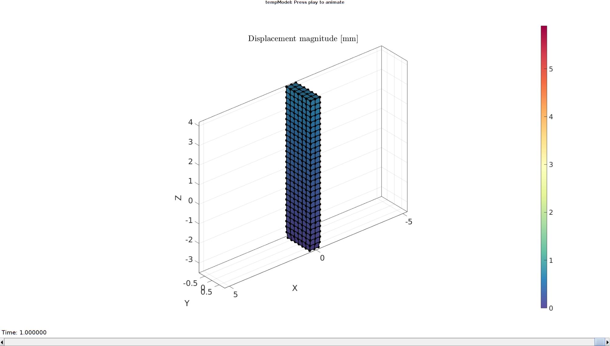
Importing element stress from a log file
    dataStruct=importFEBio_logfile(fullfile(savePath,febioLogFileName_vol),0,1);

    %Access data
    E_J_mat=dataStruct.data;
    E_J_mat(:,:,1)=1;
Plotting the simulated results using anim8 to visualize and animate deformations
    [CV]=faceToVertexMeasure(E,V,E_J_mat(:,:,end));

    % Create basic view and store graphics handle to initiate animation
    hf=cFigure; %Open figure  /usr/local/MATLAB/R2020a/bin/glnxa64/jcef_helper: symbol lookup error: /lib/x86_64-linux-gnu/libpango-1.0.so.0: undefined symbol: g_ptr_array_copy

    gtitle([febioFebFileNamePart,': Press play to animate']);
    title('$J$ [.]','Interpreter','Latex')
    hp=gpatch(Fb,V_DEF(:,:,end),CV,'k',1,2); %Add graphics object to animate
    hp.Marker='.';
    hp.MarkerSize=markerSize2;
    hp.FaceColor='interp';
    gpatch(Fb,V,0.5*ones(1,3),'none',0.25); %A static graphics object

    axisGeom(gca,fontSize);
    colormap(cMap); colorbar;
    caxis([min(E_J_mat(:)) max(E_J_mat(:))]);
    axis(axisLim(V_DEF)); %Set axis limits statically
    view(140,30);
    camlight headlight;

    % Set up animation features
    animStruct.Time=timeVec; %The time vector
    for qt=1:1:size(N_disp_mat,3) %Loop over time increments

        [CV]=faceToVertexMeasure(E,V,E_J_mat(:,:,qt));

        %Set entries in animation structure
        animStruct.Handles{qt}=[hp hp]; %Handles of objects to animate
        animStruct.Props{qt}={'Vertices','CData'}; %Properties of objects to animate
        animStruct.Set{qt}={V_DEF(:,:,qt),CV}; %Property values for to set in order to animate
    end
    anim8(hf,animStruct); %Initiate animation feature
    drawnow;
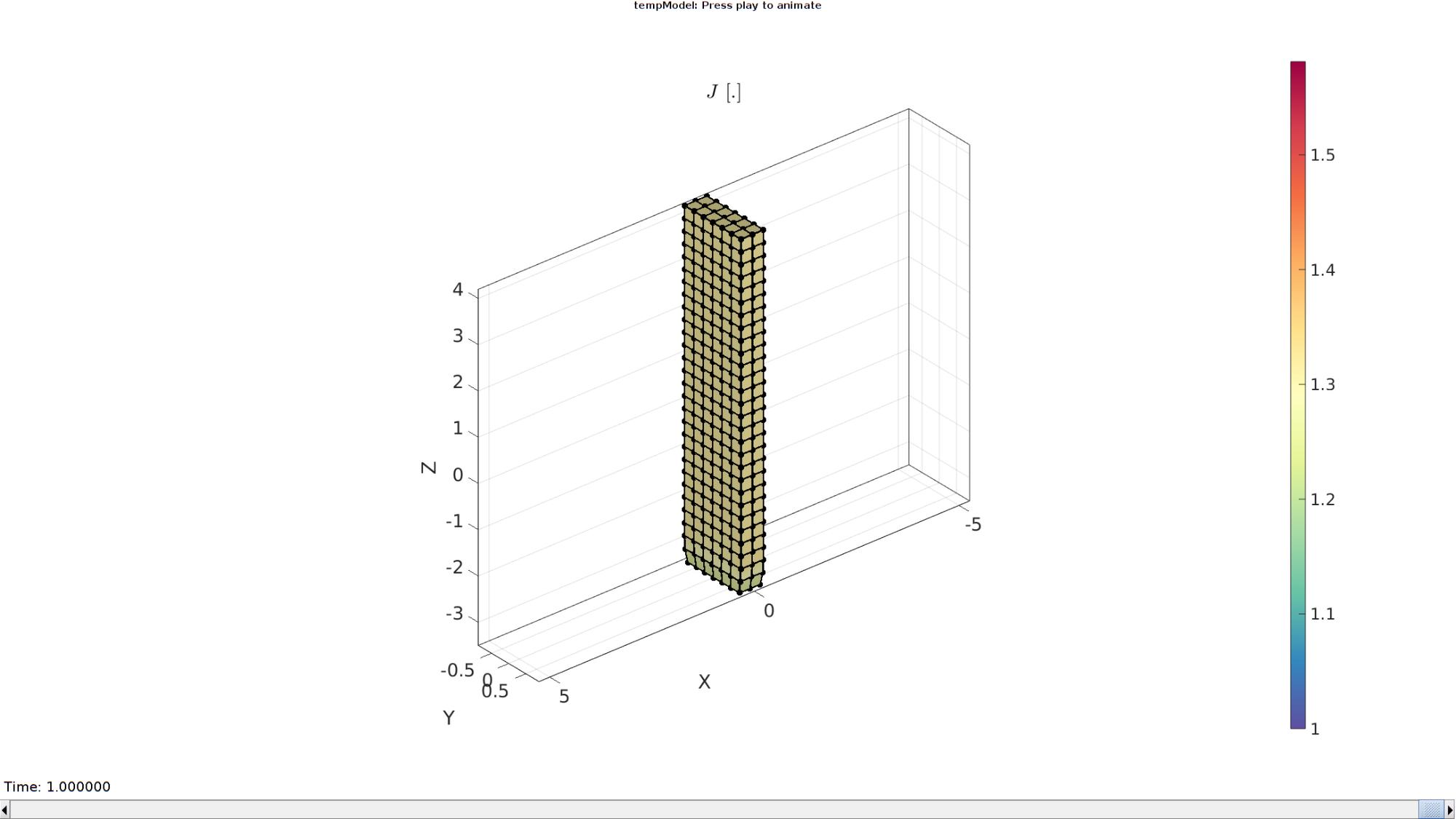
end

GIBBON www.gibboncode.org
Kevin Mattheus Moerman, [email protected]
GIBBON footer text
License: https://github.com/gibbonCode/GIBBON/blob/master/LICENSE
GIBBON: The Geometry and Image-based Bioengineering add-On. A toolbox for image segmentation, image-based modeling, meshing, and finite element analysis.
Copyright (C) 2006-2022 Kevin Mattheus Moerman and the GIBBON contributors
This program is free software: you can redistribute it and/or modify it under the terms of the GNU General Public License as published by the Free Software Foundation, either version 3 of the License, or (at your option) any later version.
This program is distributed in the hope that it will be useful, but WITHOUT ANY WARRANTY; without even the implied warranty of MERCHANTABILITY or FITNESS FOR A PARTICULAR PURPOSE. See the GNU General Public License for more details.
You should have received a copy of the GNU General Public License along with this program. If not, see http://www.gnu.org/licenses/.