DEMO_febio_0062_femur_load_01

Below is a demonstration for:

Building geometry femur bone
Applying a load to the femur head

Keywords
Plot settings
Control parameters
Import bone surface model
Scale and reorient
Visualize bone surface
Determining femur length and person's height
Cut bone surface
Visualize bone surface
Mesh using tetgen
Visualize interior point
Define material regions in bone
Visualizing solid mesh
Find femoral head
Work out force distribution on femoral head surface nodes
Marking muscle locations
Muscle force definition
Defining prescribed forces
Visualizing boundary conditions
Defining the FEBio input structure
Quick viewing of the FEBio input file structure
Exporting the FEBio input file
Running the FEBio analysis
Import FEBio results
Saving strain energy data for comparison in implant demo

Keywords

febio_spec version 4.0
febio, FEBio
beam force loading
force control boundary condition
tetrahedral elements, tet4
femur
static, solid
displacement logfile
stress logfile

clear; close all; clc;

Plot settings

fontSize=20;
faceAlpha1=0.8;
markerSize=40;
markerSize2=20;
lineWidth=3;

Control parameters

% Path names
defaultFolder = fileparts(fileparts(mfilename('fullpath')));
savePath=fullfile(defaultFolder,'data','temp');
pathNameSTL=fullfile(defaultFolder,'data','STL');
saveName_SED=fullfile(savePath,'SED_no_implant.mat');

% Defining file names
febioFebFileNamePart='tempModel';
febioFebFileName=fullfile(savePath,[febioFebFileNamePart,'.feb']); %FEB file name
febioLogFileName=[febioFebFileNamePart,'.txt']; %FEBio log file name
febioLogFileName_disp=[febioFebFileNamePart,'_disp_out.txt']; %Log file name for exporting displacement
febioLogFileName_force=[febioFebFileNamePart,'_force_out.txt']; %Log file name for exporting force
febioLogFileName_stress=[febioFebFileNamePart,'_stress_out.txt']; %Log file name for exporting stresses
febioLogFileName_strainEnergy=[febioFebFileNamePart,'_energy_out.txt']; %Log file name for exporting strain energy density

%Geometric parameters
distanceCut=250; %Distance from femur to cut bone at
corticalThickness=3; %Thickness used for cortical material definition
volumeFactor=2; %Factor to scale desired volume for interior elements w.r.t. boundary elements

%Define applied force

forceAbductor=[564.831 -132.696 704.511];
forceVastusLateralis_Walking=[-7.857 -161.505 -811.017];
forceVastusLateralis_StairClimbing=[-19.206 -195.552 -1,179.423];
forceVastusMedialis_StairClimbing=[-76.824 -345.708 -2,331.783];
forceVM_inactive=[0 0 0];

n=1;
switch n
    case 1
        forceVastusLateralis=forceVastusLateralis_Walking;
        forceVastusMedialis=forceVM_inactive;
    case 2
        forceVastusLateralis=forceVastusLateralis_StairClimbing;
        forceVastusMedialis=forceVastusMedialis_StairClimbing;
    otherwise
        forceVastusLateralis=forceVastusLateralis_StairClimbing;
        forceVastusMedialis=forceVastusMedialis_StairClimbing;
end
% Distance markers and scaling factor
zLevelWidthMeasure = -75;
zLevelFCML = -395;
scaleFactorSize=1;
distanceMuscleAttachAbductor=15;
distanceMuscleVastusLateralis=10;
distanceMuscleAttachVastusMedialis=10;

%Material parameters (MPa if spatial units are mm)
% Cortical bone
E_youngs1=17000; %Youngs modulus
nu1=0.25; %Poissons ratio

% Cancellous bone
E_youngs2=1500; %Youngs modulus
nu2=0.25; %Poissons ratio

% FEA control settings
numTimeSteps=10; %Number of time steps desired
max_refs=25; %Max reforms
max_ups=0; %Set to zero to use full-Newton iterations
opt_iter=6; %Optimum number of iterations
max_retries=5; %Maximum number of retires
dtmin=(1/numTimeSteps)/100; %Minimum time step size
dtmax=1/numTimeSteps; %Maximum time step size
runMode='external'; %'external' or 'internal'

Import bone surface model

[stlStruct] = import_STL(fullfile(pathNameSTL,'femur_iso.stl'));
F_bone=stlStruct.solidFaces{1}; %Faces
V_bone=stlStruct.solidVertices{1}; %Vertices

Scale and reorient

V_bone=V_bone.*1000; %Scale to mm
V_bone=V_bone.*scaleFactorSize; %Scale size further

[F_bone,V_bone]=mergeVertices(F_bone,V_bone); % Merging nodes
Q1=euler2DCM([0 0 0.065*pi]);
V_bone=V_bone*Q1;
Q2=euler2DCM([-0.5*pi 0 0]);
V_bone=V_bone*Q2;
Q3=euler2DCM([0 0 0.36*pi]);
V_bone=V_bone*Q3;

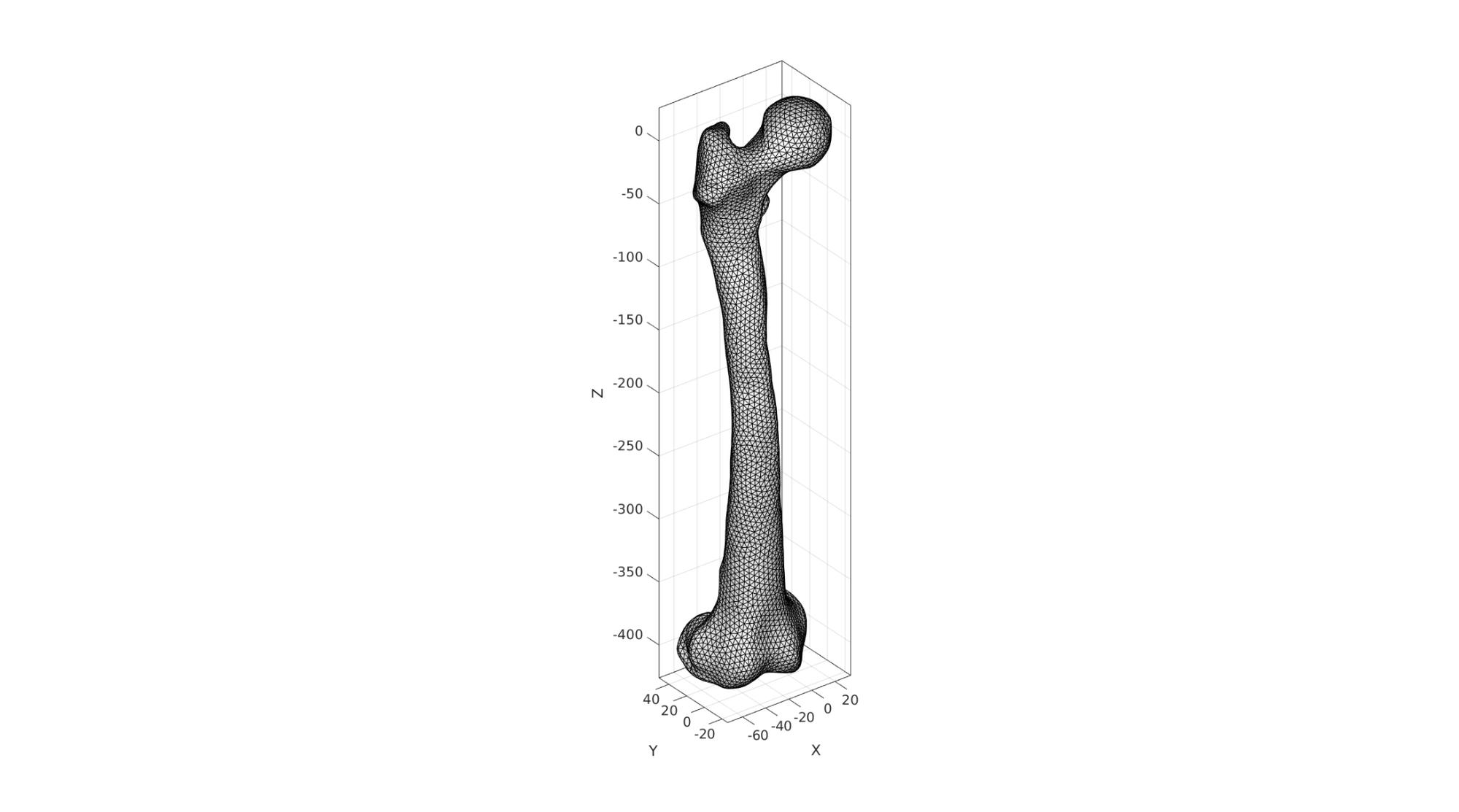
Visualize bone surface

cFigure; hold on;
gpatch(F_bone,V_bone,'w','k',1);
% patchNormPlot(F_bone,V_bone)
axisGeom; camlight headlight;
drawnow;

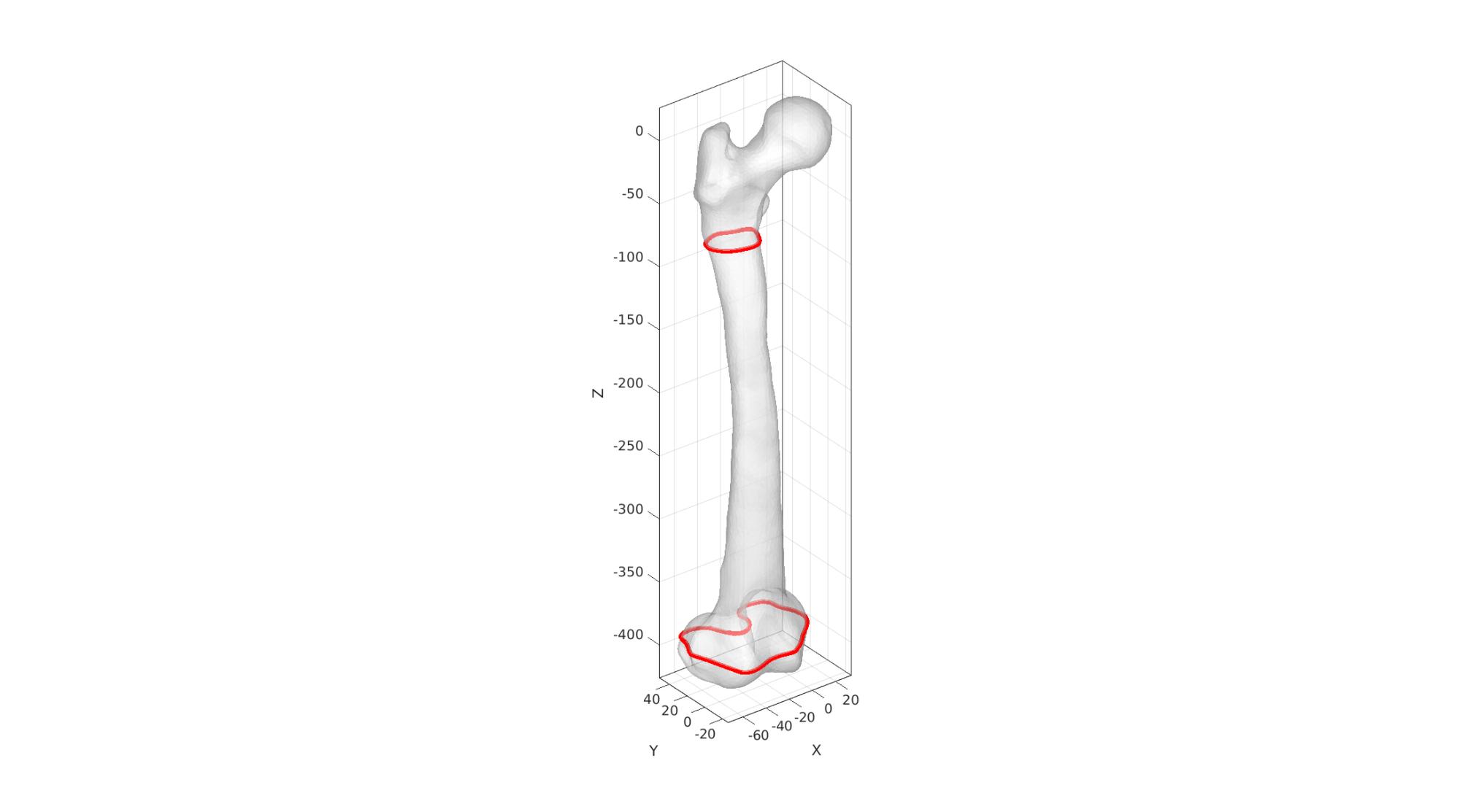
Determining femur length and person's height

% The Estimation of Stature on the Basis of Measurements of the Femur - height
% Estimating body mass and composition from proximal femur dimensions using dual energy x-ray absorptiometry - weight

% P3 = [-15 20 -75];
% [~,indNode3]=minDist(P3,V_bone);

femurLength = max(V_bone(:,3)) - min(V_bone(:,3)); %femur length

[~,V_bone_slice,~,~,Eb]=triSurfSlice(F_bone,V_bone,[],[0 0 scaleFactorSize.*zLevelWidthMeasure],[0 0 1]);
indSliceCurve=edgeListToCurve(Eb);
V_slice_curve=V_bone_slice(indSliceCurve,:);
sliceArea = polyarea(V_slice_curve(:,1),V_slice_curve(:,2));
subtrochanterMedLatDia = sqrt(sliceArea./(0.25*pi));

[~,V_bone_slice_bottom,~,~,Eb2]=triSurfSlice(F_bone,V_bone,[],[0 0 scaleFactorSize.*zLevelFCML],[0 0 1]);
indSliceCurveBottom=edgeListToCurve(Eb2);
V_slice_curve_bottom=V_bone_slice_bottom(indSliceCurveBottom,:);
sliceAreaBottom = polyarea(V_slice_curve_bottom(:,1),V_slice_curve_bottom(:,1));

FCML = max(V_bone_slice_bottom(:,1)) - min(V_bone_slice_bottom(:,1)); %mediolateral breadth of the articular surface of the femoral condyles

% subtrochanterMedLatDia = distND(V_bone(indNode3,:),V_bone(indNode4,:)); %subtrochanter medio-latreal diameter

bodyHeight = 4*femurLength;
bodyMass = 1.37 * (FCML-42.8);

forceTotal=[-0.54 -0.32  -2.292].*bodyMass;

cFigure; hold on;
gpatch(F_bone,V_bone,'w','none',0.5);
plotV(V_bone_slice(indSliceCurve,:),'r-','LineWidth',5)
plotV(V_bone_slice_bottom(indSliceCurveBottom,:),'r-','LineWidth',5)
axisGeom;
camlight headlight;
drawnow;

Cut bone surface

%Slicing surface

[F_bone,V_bone,~,logicSide,~]=triSurfSlice(F_bone,V_bone,[],[0 0 -distanceCut],[0 0 1]);

F_bone=F_bone(logicSide==0,:);
[F_bone,V_bone]=patchCleanUnused(F_bone,V_bone);

Eb=patchBoundary(F_bone,V_bone);
indCurve=edgeListToCurve(Eb);
indCurve=indCurve(1:end-1);

cparSmooth.n=5;
cparSmooth.Method='HC';
[V_Eb_smooth]=patchSmooth(Eb,V_bone(:,[1 2]),[],cparSmooth);
V_bone(indCurve,[1 2])=V_Eb_smooth(indCurve,:);

cparSmooth.n=5;
cparSmooth.Method='HC';
cparSmooth.RigidConstraints=indCurve;
[V_bone]=patchSmooth(F_bone,V_bone,[],cparSmooth);

pointSpacing=mean(patchEdgeLengths(F_bone,V_bone));

[F_bone2,V_bone2]=regionTriMesh3D({V_bone(indCurve,:)},pointSpacing,0,'linear');
if dot(mean(patchNormal(F_bone2,V_bone2)),[0 0 1])>0
    F_bone2=fliplr(F_bone2);
end

[F_bone,V_bone,C_bone]=joinElementSets({F_bone,F_bone2},{V_bone,V_bone2});
[F_bone,V_bone]=mergeVertices(F_bone,V_bone);

Warning: Second input (vertices) no longer required. Update code to avoid future
error.

Visualize bone surface

cFigure; hold on;
gpatch(F_bone,V_bone,C_bone,'k',1);
patchNormPlot(F_bone,V_bone);
axisGeom; camlight headlight;
drawnow;

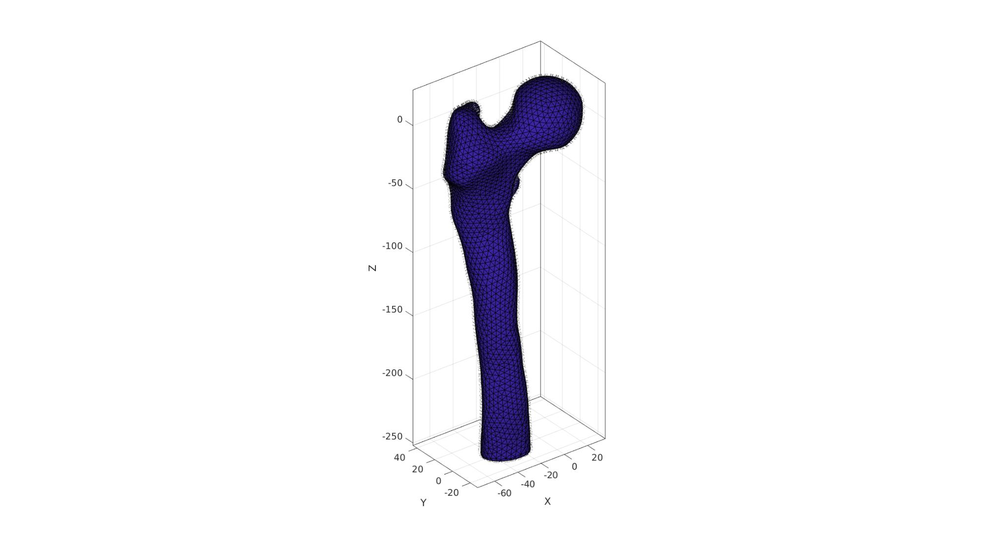
Mesh using tetgen

%Find interior point
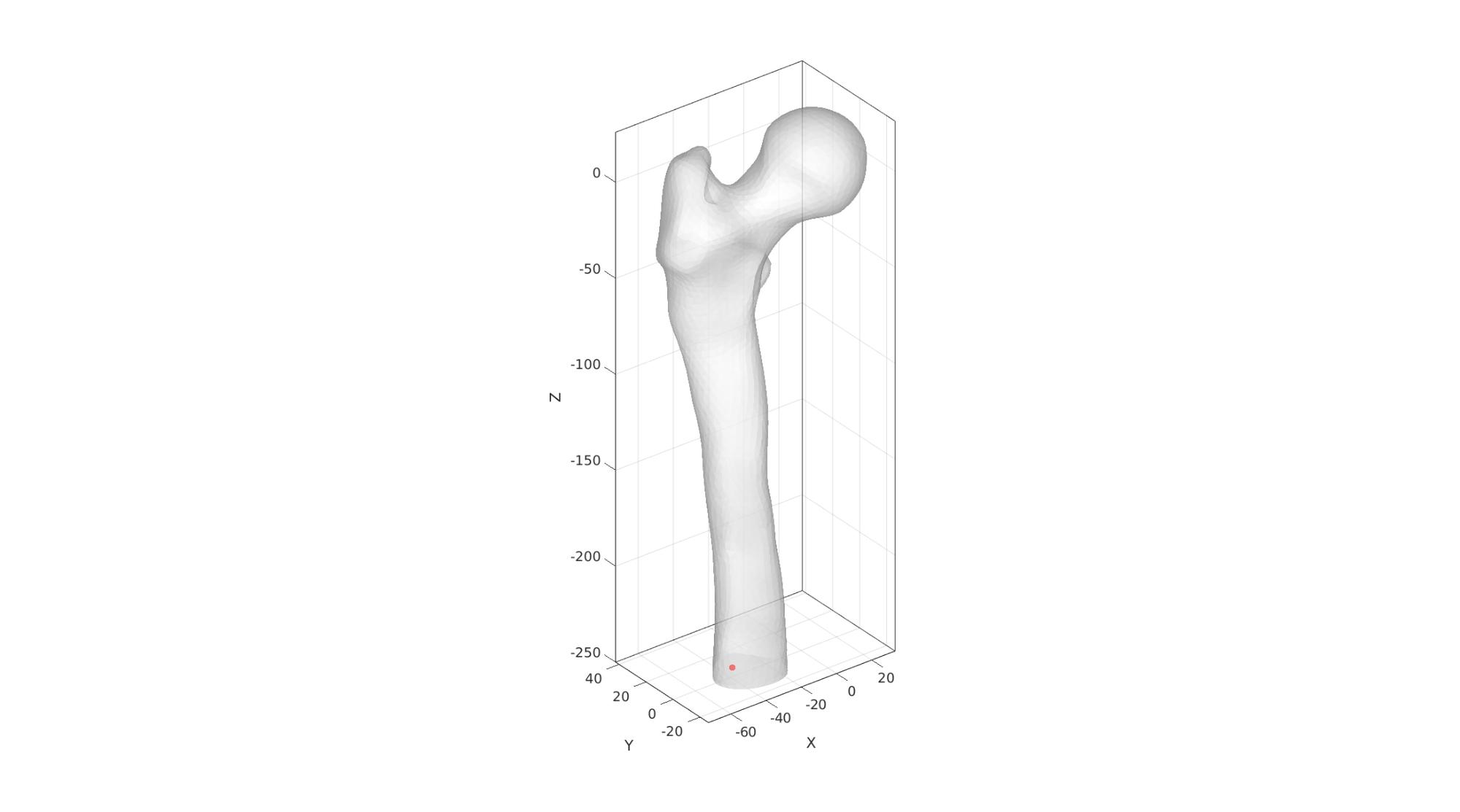
V_inner_bone=getInnerPoint(F_bone,V_bone);

Visualize interior point

cFigure; hold on;
gpatch(F_bone,V_bone,'w','none',0.5);
plotV(V_inner_bone,'r.','MarkerSize',25)
axisGeom; camlight headlight;
drawnow;

Regional mesh volume parameter

tetVolume=tetVolMeanEst(F_bone,V_bone); %Volume for regular tets

tetGenStruct.stringOpt='-pq1.2AaY';
tetGenStruct.Faces=F_bone;
tetGenStruct.Nodes=V_bone;
tetGenStruct.holePoints=[];
tetGenStruct.faceBoundaryMarker=C_bone; %Face boundary markers
tetGenStruct.regionPoints=V_inner_bone; %region points
tetGenStruct.regionA=tetVolume*volumeFactor;

[meshOutput]=runTetGen(tetGenStruct); %Run tetGen

% Access elements, nodes, and boundary faces
E=meshOutput.elements;
V=meshOutput.nodes;
Fb=meshOutput.facesBoundary;
Cb=meshOutput.boundaryMarker;
CE=meshOutput.elementMaterialID;

 
%%%%%%%%%%%%%%%%%%%%%%%%%%%%%%%%%%%%%%%%%%%%%
--- TETGEN Tetrahedral meshing --- 29-May-2023 10:36:56
 
%%%%%%%%%%%%%%%%%%%%%%%%%%%%%%%%%%%%%%%%%%%%%
--- Writing SMESH file --- 29-May-2023 10:36:56
----> Adding node field
----> Adding facet field
----> Adding holes specification
----> Adding region specification
--- Done --- 29-May-2023 10:36:56
--- Running TetGen to mesh input boundary--- 29-May-2023 10:36:56
Opening /home/kevin/DATA/Code/matlab/GIBBON/data/temp/temp.smesh.
Delaunizing vertices...
Delaunay seconds:  0.009426
Creating surface mesh ...
Surface mesh seconds:  0.002424
Recovering boundaries...
Boundary recovery seconds:  0.00449
Removing exterior tetrahedra ...
Spreading region attributes.
Exterior tets removal seconds:  0.002639
Recovering Delaunayness...
Delaunay recovery seconds:  0.002175
Refining mesh...
  3940 insertions, added 3883 points, 119011 tetrahedra in queue.
  1312 insertions, added 1213 points, 44212 tetrahedra in queue.
Refinement seconds:  0.063345
Smoothing vertices...
Mesh smoothing seconds:  0.121055
Improving mesh...
Mesh improvement seconds:  0.004366

Writing /home/kevin/DATA/Code/matlab/GIBBON/data/temp/temp.1.node.
Writing /home/kevin/DATA/Code/matlab/GIBBON/data/temp/temp.1.ele.
Writing /home/kevin/DATA/Code/matlab/GIBBON/data/temp/temp.1.face.
Writing /home/kevin/DATA/Code/matlab/GIBBON/data/temp/temp.1.edge.

Output seconds:  0.018217
Total running seconds:  0.228312

Statistics:

  Input points: 2956
  Input facets: 5908
  Input segments: 8862
  Input holes: 0
  Input regions: 1

  Mesh points: 8138
  Mesh tetrahedra: 40574
  Mesh faces: 84102
  Mesh faces on exterior boundary: 5908
  Mesh faces on input facets: 5908
  Mesh edges on input segments: 8862
  Steiner points inside domain: 5182

--- Done --- 29-May-2023 10:36:56
 
%%%%%%%%%%%%%%%%%%%%%%%%%%%%%%%%%%%%%%%%%%%%%
--- Importing TetGen files --- 29-May-2023 10:36:56
--- Done --- 29-May-2023 10:36:56

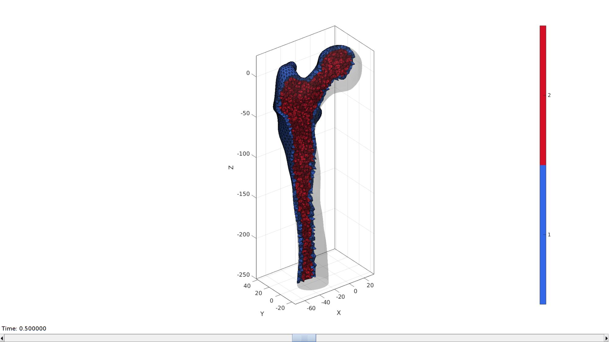
Define material regions in bone

indBoundary=unique(Fb(Cb==1,:));
DE=minDist(V,V(indBoundary,:));
logicCorticalNodes=DE<=corticalThickness;
logicCorticalElements=any(logicCorticalNodes(E),2);
logicCancellousElements=~logicCorticalElements;

E1=E(logicCorticalElements,:);
E2=E(logicCancellousElements,:);
E=[E1;E2];
elementMaterialID=[ones(size(E1,1),1);2*ones(size(E2,1),1);];
meshOutput.elements=E;
meshOutput.elementMaterialID=elementMaterialID;

Visualizing solid mesh

hFig=cFigure; hold on;
optionStruct.hFig=hFig;
meshView(meshOutput,optionStruct);
axisGeom;
drawnow;

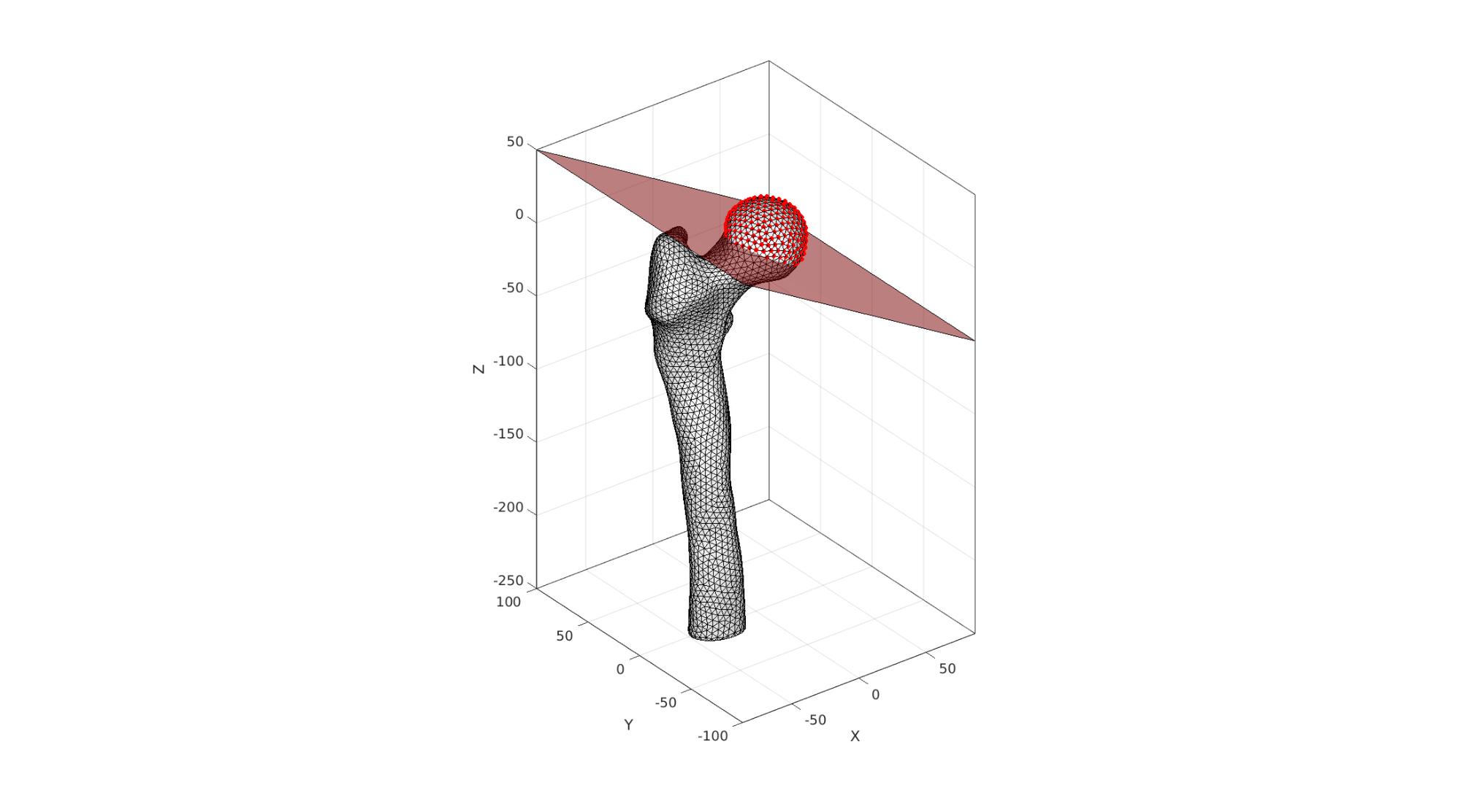
Find femoral head

w=100;
f=[1 2 3 4];
v=w*[-1 -1 0; -1 1 0; 1 1 0; 1 -1 0];

p=[0 0 0];
Q=euler2DCM([0 (150/180)*pi 0]);
v=v*Q;
v=v+p;

Vr=V*Q';
Vr=Vr+p;
logicHeadNodes=Vr(:,3)<0;
logicHeadFaces=all(logicHeadNodes(Fb),2);
bcPrescribeList_head=unique(Fb(logicHeadFaces,:));

Visualize femoral head nodes for prescribed force boundary conditions

cFigure;
hold on;
gpatch(Fb,V,'w','k',1);
gpatch(f,v,'r','k',0.5);
plotV(V(bcPrescribeList_head,:),'r.','markerSize',15)
axisGeom; camlight headlight;
drawnow;

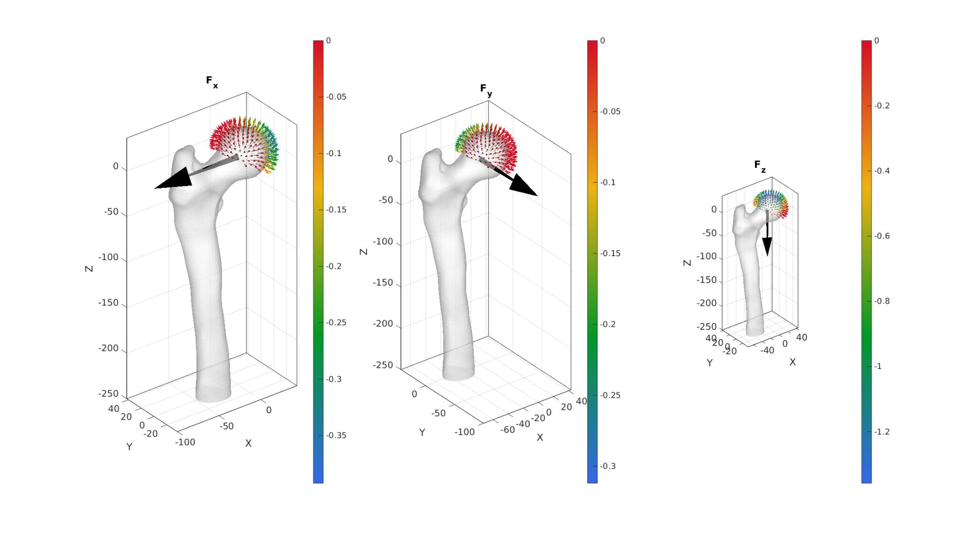
Work out force distribution on femoral head surface nodes

This is based on surface normal directions. Forces are assumed to only be able to act in a compressive sense on the bone.

[~,~,N]=patchNormal(fliplr(Fb),V); %Nodal normal directions

FX=[forceTotal(1) 0 0]; %X force vector
FY=[0 forceTotal(2) 0]; %Y force vector
FZ=[0 0 forceTotal(3)]; %Z force vector

wx=dot(N(bcPrescribeList_head,:),FX(ones(numel(bcPrescribeList_head),1),:),2);
wy=dot(N(bcPrescribeList_head,:),FY(ones(numel(bcPrescribeList_head),1),:),2);
wz=dot(N(bcPrescribeList_head,:),FZ(ones(numel(bcPrescribeList_head),1),:),2);

%Force zero
wx(wx>0)=0; wy(wy>0)=0; wz(wz>0)=0;

force_X=forceTotal(1).*ones(numel(bcPrescribeList_head),1).*wx;
force_Y=forceTotal(2).*ones(numel(bcPrescribeList_head),1).*wy;
force_Z=forceTotal(3).*ones(numel(bcPrescribeList_head),1).*wz;

force_X=force_X./sum(force_X(:)); %sum now equal to 1
force_X=force_X.*forceTotal(1); %sum now equal to desired

force_Y=force_Y./sum(force_Y(:)); %sum now equal to 1
force_Y=force_Y.*forceTotal(2); %sum now equal to desired

force_Z=force_Z./sum(force_Z(:)); %sum now equal to 1
force_Z=force_Z.*forceTotal(3); %sum now equal to desired

force_head=[force_X(:) force_Y(:) force_Z(:)];

cFigure;
subplot(1,3,1);hold on;
title('F_x');
gpatch(Fb,V,'w','none',0.5);
quiverVec([0 0 0],FX,100,'k');
% scatterV(V(indicesHeadNodes,:),15)
quiverVec(V(bcPrescribeList_head,:),N(bcPrescribeList_head,:),10,force_X);
axisGeom; camlight headlight;
colormap(gca,gjet(250)); colorbar;

subplot(1,3,2);hold on;
title('F_y');
gpatch(Fb,V,'w','none',0.5);
quiverVec([0 0 0],FY,100,'k');
% scatterV(V(indicesHeadNodes,:),15)
quiverVec(V(bcPrescribeList_head,:),N(bcPrescribeList_head,:),10,force_Y);
axisGeom; camlight headlight;
colormap(gca,gjet(250)); colorbar;

subplot(1,3,3);hold on;
title('F_z');
gpatch(Fb,V,'w','none',0.5);
quiverVec([0 0 0],FZ,100,'k');
% scatterV(V(indicesHeadNodes,:),15)
quiverVec(V(bcPrescribeList_head,:),N(bcPrescribeList_head,:),10,force_Z);
axisGeom; camlight headlight;
colormap(gca,gjet(250)); colorbar;

drawnow;

Marking muscle locations

P_abductor_find = [-69.771045288206111 8.185179717034659 -5.575329878303917]; %Coordinate at centre of muscle attachment
[~,indAbductor]=minDist(P_abductor_find,V); %Node number of point at centre of attachment
dAbductor=meshDistMarch(Fb,V,indAbductor); %Distance (on mesh) from attachement centre
bcPrescibeList_abductor=find(dAbductor<=distanceMuscleAttachAbductor); %Node numbers for attachment site

P_VastusLateralis_find = [-58.763839901506827 19.145444610053566 -51.005278396808819]; %Coordinate at centre of muscle attachment
[~,indVastusLateralis]=minDist(P_VastusLateralis_find,V); %Node number of point at centre of attachment
dVastusLateralis=meshDistMarch(Fb,V,indVastusLateralis); %Distance (on mesh) from attachement centre
bcPrescibeList_VastusLateralis=find(dVastusLateralis<=distanceMuscleVastusLateralis); %Node numbers for attachment site


P_VastusMedialis_find = [-18.533631492778085 9.501312355952791 -85.666499329588035]; %Coordinate at centre of muscle attachment
[~,indVastusMedialis]=minDist(P_VastusMedialis_find,V); %Node number of point at centre of attachment
dVastusMedialis=meshDistMarch(Fb,V,indVastusMedialis); %Distance (on mesh) from attachement centre
bcPrescibeList_VastusMedialis=find(dVastusMedialis<=distanceMuscleAttachVastusMedialis); %Node numbers for attachment site

Muscle force definition

forceAbductor_distributed=forceAbductor.*ones(numel(bcPrescibeList_abductor),1)./numel(bcPrescibeList_abductor);

forceVastusLateralis_distributed=forceVastusLateralis.*ones(numel(bcPrescibeList_VastusLateralis),1)./numel(bcPrescibeList_VastusLateralis);

forceVastusMedialis_distributed=forceVastusMedialis.*ones(numel(bcPrescibeList_VastusMedialis),1)./numel(bcPrescibeList_VastusMedialis);

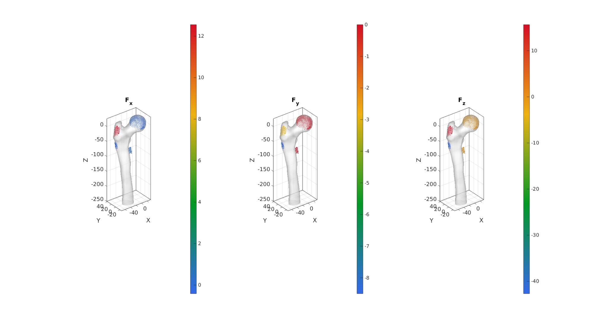
Defining prescribed forces

bcPrescribeList=[bcPrescribeList_head(:);...
                 bcPrescibeList_abductor(:);...
                 bcPrescibeList_VastusLateralis(:);...
                 bcPrescibeList_VastusMedialis(:)];

forceData=[force_head;...
           forceAbductor_distributed;...
           forceVastusLateralis_distributed;...
           forceVastusMedialis_distributed];

cFigure;
subplot(1,3,1);hold on;
title('F_x');
gpatch(Fb,V,'w','none',0.5);
quiverVec(V(bcPrescribeList,:),forceData,10,forceData(:,1));
axisGeom; camlight headlight;
colormap(gca,gjet(250)); colorbar;

subplot(1,3,2);hold on;
title('F_y');
gpatch(Fb,V,'w','none',0.5);
quiverVec(V(bcPrescribeList,:),forceData,10,forceData(:,2));
axisGeom; camlight headlight;
colormap(gca,gjet(250)); colorbar;

subplot(1,3,3);hold on;
title('F_z');
gpatch(Fb,V,'w','none',0.5);

quiverVec(V(bcPrescribeList,:),forceData,10,forceData(:,3));
axisGeom; camlight headlight;
colormap(gca,gjet(250)); colorbar;

drawnow;

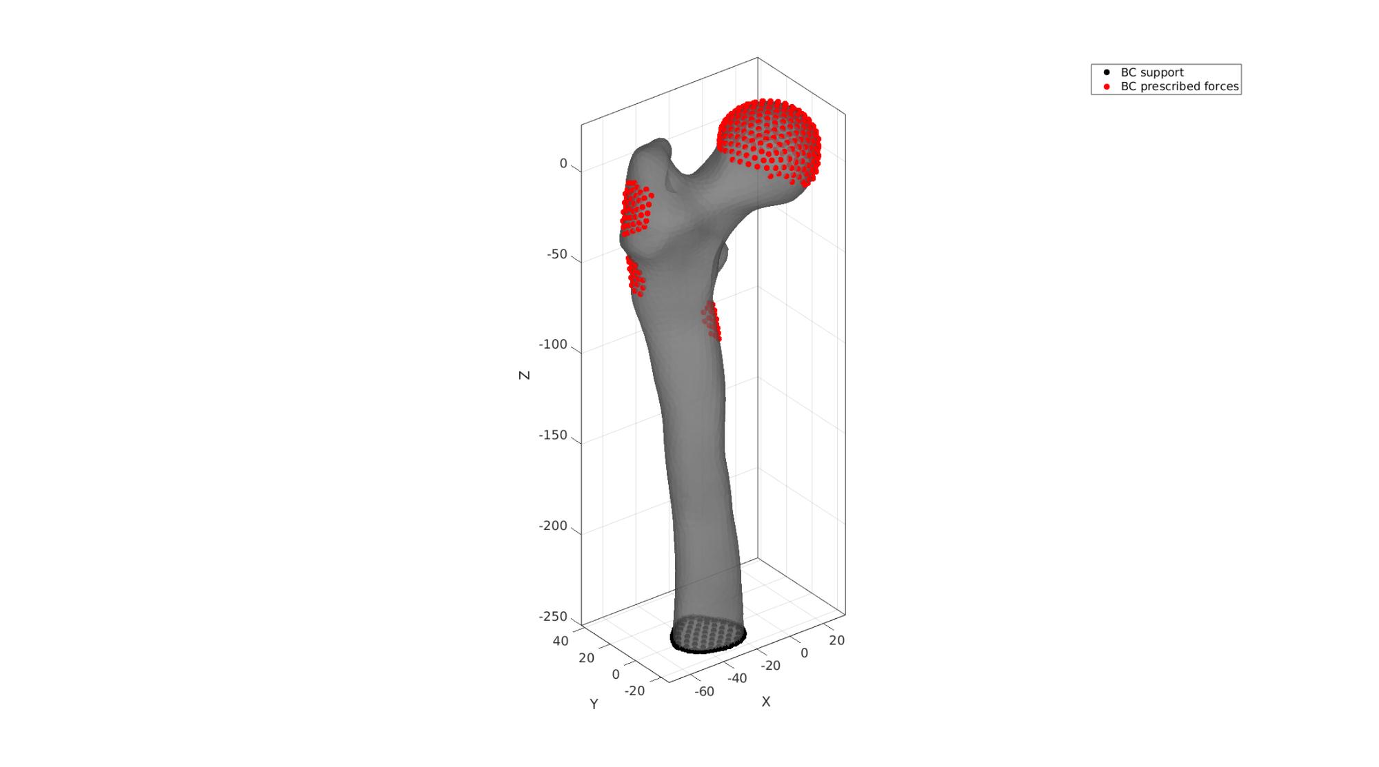
Visualizing boundary conditions

F_bottomSupport=Fb(Cb==2,:);
bcSupportList=unique(F_bottomSupport(:));

cFigure; hold on;
gpatch(Fb,V,'kw','none',0.7);
hl(1)=plotV(V(bcSupportList,:),'k.','MarkerSize',25);
hl(2)=plotV(V(bcPrescribeList,:),'r.','MarkerSize',25);

legend(hl,{'BC support','BC prescribed forces'});
axisGeom;
camlight headlight;
drawnow;

Defining the FEBio input structure

See also febioStructTemplate and febioStruct2xml and the FEBio user manual.

%Get a template with default settings
[febio_spec]=febioStructTemplate;

%febio_spec version
febio_spec.ATTR.version='4.0';

%Module section
febio_spec.Module.ATTR.type='solid';

%Control section
febio_spec.Control.analysis='STATIC';
febio_spec.Control.time_steps=numTimeSteps;
febio_spec.Control.step_size=1/numTimeSteps;
febio_spec.Control.solver.max_refs=max_refs;
febio_spec.Control.solver.qn_method.max_ups=max_ups;
febio_spec.Control.time_stepper.dtmin=dtmin;
febio_spec.Control.time_stepper.dtmax=dtmax;
febio_spec.Control.time_stepper.max_retries=max_retries;
febio_spec.Control.time_stepper.opt_iter=opt_iter;

%Material section
materialName1='Material1';
febio_spec.Material.material{1}.ATTR.name=materialName1;
febio_spec.Material.material{1}.ATTR.type='neo-Hookean';
febio_spec.Material.material{1}.ATTR.id=1;
febio_spec.Material.material{1}.E=E_youngs1;
febio_spec.Material.material{1}.v=nu1;

materialName2='Material2';
febio_spec.Material.material{2}.ATTR.name=materialName2;
febio_spec.Material.material{2}.ATTR.type='neo-Hookean';
febio_spec.Material.material{2}.ATTR.id=2;
febio_spec.Material.material{2}.E=E_youngs2;
febio_spec.Material.material{2}.v=nu2;

% Mesh section
% -> Nodes
febio_spec.Mesh.Nodes{1}.ATTR.name='Object1'; %The node set name
febio_spec.Mesh.Nodes{1}.node.ATTR.id=(1:size(V,1))'; %The node id's
febio_spec.Mesh.Nodes{1}.node.VAL=V; %The nodel coordinates

% -> Elements
partName1='CorticalBone';
febio_spec.Mesh.Elements{1}.ATTR.name=partName1; %Name of this part
febio_spec.Mesh.Elements{1}.ATTR.type='tet4'; %Element type
febio_spec.Mesh.Elements{1}.elem.ATTR.id=(1:1:size(E1,1))'; %Element id's
febio_spec.Mesh.Elements{1}.elem.VAL=E1; %The element matrix

partName2='CancellousBone';
febio_spec.Mesh.Elements{2}.ATTR.name=partName2; %Name of this part
febio_spec.Mesh.Elements{2}.ATTR.type='tet4'; %Element type
febio_spec.Mesh.Elements{2}.elem.ATTR.id=size(E1,1)+(1:1:size(E2,1))'; %Element id's
febio_spec.Mesh.Elements{2}.elem.VAL=E2; %The element matrix

% -> NodeSets
nodeSetName1='bcSupportList';
febio_spec.Mesh.NodeSet{1}.ATTR.name=nodeSetName1;
febio_spec.Mesh.NodeSet{1}.VAL=mrow(bcSupportList);

nodeSetName2='bcPrescribeList';
febio_spec.Mesh.NodeSet{2}.ATTR.name=nodeSetName2;
febio_spec.Mesh.NodeSet{2}.VAL=mrow(bcPrescribeList);

%MeshDomains section
febio_spec.MeshDomains.SolidDomain{1}.ATTR.name=partName1;
febio_spec.MeshDomains.SolidDomain{1}.ATTR.mat=materialName1;

febio_spec.MeshDomains.SolidDomain{2}.ATTR.name=partName2;
febio_spec.MeshDomains.SolidDomain{2}.ATTR.mat=materialName2;

%Boundary condition section
% -> Fix boundary conditions
febio_spec.Boundary.bc{1}.ATTR.name='zero_displacement_xyz';
febio_spec.Boundary.bc{1}.ATTR.type='zero displacement';
febio_spec.Boundary.bc{1}.ATTR.node_set=nodeSetName1;
febio_spec.Boundary.bc{1}.x_dof=1;
febio_spec.Boundary.bc{1}.y_dof=1;
febio_spec.Boundary.bc{1}.z_dof=1;

%MeshData secion
%-> Node data
loadDataName1='nodal_forces';
febio_spec.MeshData.NodeData{1}.ATTR.name=loadDataName1;
febio_spec.MeshData.NodeData{1}.ATTR.node_set=nodeSetName2;
febio_spec.MeshData.NodeData{1}.ATTR.data_type='vec3';
febio_spec.MeshData.NodeData{1}.node.ATTR.lid=(1:1:numel(bcPrescribeList))';
febio_spec.MeshData.NodeData{1}.node.VAL=forceData;

%Loads section
% -> Prescribed nodal forces
febio_spec.Loads.nodal_load{1}.ATTR.name='PrescribedForce';
febio_spec.Loads.nodal_load{1}.ATTR.type='nodal_force';
febio_spec.Loads.nodal_load{1}.ATTR.node_set=nodeSetName2;
febio_spec.Loads.nodal_load{1}.value.ATTR.lc=1;
febio_spec.Loads.nodal_load{1}.value.ATTR.type='map';
febio_spec.Loads.nodal_load{1}.value.VAL=loadDataName1;

%LoadData section
% -> load_controller
febio_spec.LoadData.load_controller{1}.ATTR.name='LC_1';
febio_spec.LoadData.load_controller{1}.ATTR.id=1;
febio_spec.LoadData.load_controller{1}.ATTR.type='loadcurve';
febio_spec.LoadData.load_controller{1}.interpolate='LINEAR';
%febio_spec.LoadData.load_controller{1}.extend='CONSTANT';
febio_spec.LoadData.load_controller{1}.points.pt.VAL=[0 0; 1 1];

%Output section
% -> log file
febio_spec.Output.logfile.ATTR.file=febioLogFileName;
febio_spec.Output.logfile.node_data{1}.ATTR.file=febioLogFileName_disp;
febio_spec.Output.logfile.node_data{1}.ATTR.data='ux;uy;uz';
febio_spec.Output.logfile.node_data{1}.ATTR.delim=',';

febio_spec.Output.logfile.element_data{1}.ATTR.file=febioLogFileName_stress;
febio_spec.Output.logfile.element_data{1}.ATTR.data='s1;s2;s3';
febio_spec.Output.logfile.element_data{1}.ATTR.delim=',';

febio_spec.Output.logfile.element_data{2}.ATTR.file=febioLogFileName_strainEnergy;
febio_spec.Output.logfile.element_data{2}.ATTR.data='sed';
febio_spec.Output.logfile.element_data{2}.ATTR.delim=',';

% Plotfile section
febio_spec.Output.plotfile.compression=0;

Quick viewing of the FEBio input file structure

The febView function can be used to view the xml structure in a MATLAB figure window.

febView(febio_spec); %Viewing the febio file

Exporting the FEBio input file

Exporting the febio_spec structure to an FEBio input file is done using the febioStruct2xml function.

febioStruct2xml(febio_spec,febioFebFileName); %Exporting to file and domNode

Running the FEBio analysis

To run the analysis defined by the created FEBio input file the runMonitorFEBio function is used. The input for this function is a structure defining job settings e.g. the FEBio input file name. The optional output runFlag informs the user if the analysis was run succesfully.

febioAnalysis.run_filename=febioFebFileName; %The input file name
febioAnalysis.run_logname=febioLogFileName; %The name for the log file
febioAnalysis.disp_on=1; %Display information on the command window
febioAnalysis.runMode=runMode;

[runFlag]=runMonitorFEBio(febioAnalysis);%START FEBio NOW!!!!!!!!

 
%%%%%%%%%%%%%%%%%%%%%%%%%%%%%%%%%%%%%%%%%%%%%%%%%%%%%%%%%%%%%%%%%%%%%%%%%%%
-------->    RUNNING/MONITORING FEBIO JOB    <-------- 29-May-2023 10:37:03
FEBio path: /home/kevin/FEBioStudio/bin/febio4
# Attempt removal of existing log files                29-May-2023 10:37:03
 * Removal succesful                                   29-May-2023 10:37:03
# Attempt removal of existing .xplt files              29-May-2023 10:37:03
 * Removal succesful                                   29-May-2023 10:37:03
# Starting FEBio...                                    29-May-2023 10:37:03
  Max. total analysis time is: Inf s
 * Waiting for log file creation                       29-May-2023 10:37:03
   Max. wait time: 30 s
 * Log file found.                                     29-May-2023 10:37:03
# Parsing log file...                                  29-May-2023 10:37:03
    number of iterations   : 3                         29-May-2023 10:37:04
    number of reformations : 3                         29-May-2023 10:37:04
------- converged at time : 0.1                        29-May-2023 10:37:04
    number of iterations   : 3                         29-May-2023 10:37:04
    number of reformations : 3                         29-May-2023 10:37:04
------- converged at time : 0.2                        29-May-2023 10:37:04
    number of iterations   : 3                         29-May-2023 10:37:05
    number of reformations : 3                         29-May-2023 10:37:05
------- converged at time : 0.3                        29-May-2023 10:37:05
    number of reformations : 3                         29-May-2023 10:37:06
------- converged at time : 0.4                        29-May-2023 10:37:06
    number of iterations   : 3                         29-May-2023 10:37:06
    number of reformations : 3                         29-May-2023 10:37:06
------- converged at time : 0.5                        29-May-2023 10:37:06
    number of iterations   : 3                         29-May-2023 10:37:08
    number of reformations : 3                         29-May-2023 10:37:08
------- converged at time : 0.6                        29-May-2023 10:37:08
    number of iterations   : 3                         29-May-2023 10:37:08
    number of reformations : 3                         29-May-2023 10:37:08
------- converged at time : 0.7                        29-May-2023 10:37:08
    number of iterations   : 3                         29-May-2023 10:37:09
    number of reformations : 3                         29-May-2023 10:37:09
------- converged at time : 0.8                        29-May-2023 10:37:09
    number of iterations   : 3                         29-May-2023 10:37:09
    number of reformations : 3                         29-May-2023 10:37:09
------- converged at time : 0.9                        29-May-2023 10:37:09
    number of iterations   : 3                         29-May-2023 10:37:10
    number of reformations : 3                         29-May-2023 10:37:10
------- converged at time : 1                          29-May-2023 10:37:10
 Elapsed time : 0:00:07                                29-May-2023 10:37:10
 N O R M A L   T E R M I N A T I O N
# Done                                                 29-May-2023 10:37:10
%%%%%%%%%%%%%%%%%%%%%%%%%%%%%%%%%%%%%%%%%%%%%%%%%%%%%%%%%%%%%%%%%%%%%%%%%%%

Import FEBio results

if runFlag==1 %i.e. a succesful run

Importing nodal displacements from a log file

    dataStruct=importFEBio_logfile(fullfile(savePath,febioLogFileName_disp),0,1);

    %Access data
    N_disp_mat=dataStruct.data; %Displacement
    timeVec=dataStruct.time; %Time

    %Create deformed coordinate set
    V_DEF=N_disp_mat+repmat(V,[1 1 size(N_disp_mat,3)]);

Importing element strain energies from a log file

    dataStruct=importFEBio_logfile(fullfile(savePath,febioLogFileName_strainEnergy),0,1); %Element strain energy

    %Access data
    E_energy=dataStruct.data;

Saving strain energy data for comparison in implant demo

    %Element centre coordinates
    VE=patchCentre(E,V);

    %Construct interpolation function
    interpFuncEnergy=scatteredInterpolant(VE,E_energy(:,:,end),'natural','linear');

    %Store components in structure
    outputStruct.SED=E_energy;
    outputStruct.elements=E;
    outputStruct.nodes=V;
    outputStruct.boundaryFaces=Fb;
    outputStruct.elementCenters=VE;
    outputStruct.interpFuncEnergy=interpFuncEnergy;

    %Save structure
    save(saveName_SED,'-struct','outputStruct');

    C_data=E_energy(:,:,end);

    n=[0 1 0]; %Normal direction to plane
    P=mean(V,1); %Point on plane
    [logicAt]=meshCleave(E,V,P,n);

    % Get faces and matching color data for visualization
    [F_cleave,CF_cleave]=element2patch(E(logicAt,:),C_data(logicAt));

    hf=cFigure; hold on;
    title('Strain energy density');
    gpatch(Fb,V,'w','none',0.1); %Add graphics object to animate

    hp1=gpatch(F_cleave,V,CF_cleave,'k',1);
    axisGeom(gca,fontSize);
    colormap(gjet(250));
    caxis([0 max(C_data)]/2);
    colorbar; axis manual;
    camlight headligth;
    gdrawnow;

    nSteps=25; %Number of animation steps

    %Create the time vector
    animStruct.Time=linspace(0,1,nSteps);

    %The vector lengths
    y=linspace(min(V(:,2)),max(V(:,2)),nSteps);
    for q=1:1:nSteps
        %Get logic for slice of elements
        logicAt=meshCleave(E,V,[0 y(q) 0],n,[1 0]);

        % Get faces and matching color data for cleaves elements
        [F_cleave,CF_cleave]=element2patch(E(logicAt,:),C_data(logicAt));

        %Set entries in animation structure
        animStruct.Handles{q}=[hp1 hp1]; %Handles of objects to animate
        animStruct.Props{q}={'Faces','CData'}; %Properties of objects to animate
        animStruct.Set{q}={F_cleave,CF_cleave}; %Property values for to set in order to animate
    end
    anim8(hf,animStruct);

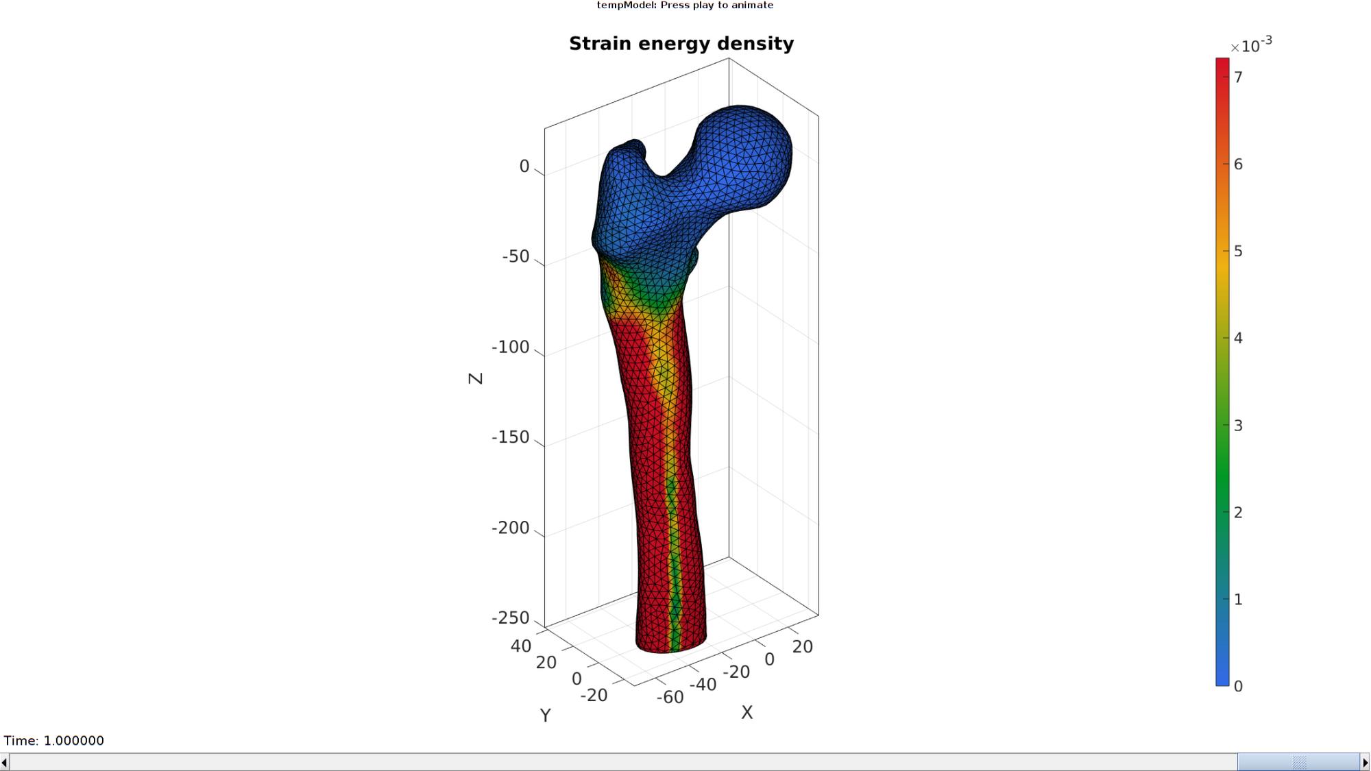
Plotting the simulated results using anim8 to visualize and animate deformations

    [CV]=faceToVertexMeasure(E,V,E_energy(:,:,end));

    % Create basic view and store graphics handle to initiate animation
    hf=cFigure; %Open figure
    title('Strain energy density')
    gtitle([febioFebFileNamePart,': Press play to animate']);
    hp1=gpatch(Fb,V_DEF(:,:,end),CV,'k',1); %Add graphics object to animate
    hp1.FaceColor='Interp';

    axisGeom(gca,fontSize);
    colormap(gjet(250)); colorbar;
    clim([0 max(E_energy(:))/25]);
    axis(axisLim(V_DEF)); %Set axis limits statically
    camlight headlight;

    % Set up animation features
    animStruct.Time=timeVec; %The time vector
    for qt=1:1:size(N_disp_mat,3) %Loop over time increments

        [CV]=faceToVertexMeasure(E,V,E_energy(:,:,qt));

        %Set entries in animation structure
        animStruct.Handles{qt}=[hp1 hp1]; %Handles of objects to animate
        animStruct.Props{qt}={'Vertices','CData'}; %Properties of objects to animate
        animStruct.Set{qt}={V_DEF(:,:,qt),CV}; %Property values for to set in order to animate
    end
    anim8(hf,animStruct); %Initiate animation feature
    drawnow;

end

GIBBON footer text

License: https://github.com/gibbonCode/GIBBON/blob/master/LICENSE

GIBBON: The Geometry and Image-based Bioengineering add-On. A toolbox for image segmentation, image-based modeling, meshing, and finite element analysis.

This program is free software: you can redistribute it and/or modify it under the terms of the GNU General Public License as published by the Free Software Foundation, either version 3 of the License, or (at your option) any later version.

This program is distributed in the hope that it will be useful, but WITHOUT ANY WARRANTY; without even the implied warranty of MERCHANTABILITY or FITNESS FOR A PARTICULAR PURPOSE. See the GNU General Public License for more details.

You should have received a copy of the GNU General Public License along with this program. If not, see http://www.gnu.org/licenses/.

DEMO_febio_0062_femur_load_01

Contents

Keywords

Plot settings

Control parameters

Import bone surface model

Scale and reorient

Visualize bone surface

Determining femur length and person's height

Cut bone surface

Visualize bone surface

Mesh using tetgen

Visualize interior point

Define material regions in bone

Visualizing solid mesh

Find femoral head

Work out force distribution on femoral head surface nodes

Marking muscle locations

Muscle force definition

Defining prescribed forces

Visualizing boundary conditions

Defining the FEBio input structure

Quick viewing of the FEBio input file structure

Exporting the FEBio input file

Running the FEBio analysis

Import FEBio results

Saving strain energy data for comparison in implant demo