DEMO_febio_0054_lattice_hydrostatic_01

Below is a demonstration for:

Building geometry for a cube with hexahedral elements
Defining the boundary conditions
Coding the febio structure
Running the model
Importing and visualizing the displacement and stress results

Keywords
Plot settings
Control parameters
Create lattice
DEFINE BC's
Smoothing lattice
Defining the FEBio input structure
Quick viewing of the FEBio input file structure
Exporting the FEBio input file
Running the FEBio analysis
Import FEBio results

Keywords

febio_spec version 4.0
febio, FEBio
uniaxial loading
compression, tension, compressive, tensile
displacement control, displacement boundary condition
hexahedral elements, hex8
cube, box, rectangular
static, solid
hyperelastic, Ogden
displacement logfile
stress logfile

clear; close all; clc;

Plot settings

fontSize=15;
faceAlpha1=0.8;
faceAlpha2=1;
edgeColor=0.25*ones(1,3);
edgeWidth=1.5;
markerSize=25;
cMap=gjet(4);

Control parameters

% Path names
defaultFolder = fileparts(fileparts(mfilename('fullpath')));
savePath=fullfile(defaultFolder,'data','temp');

% Defining file names
febioFebFileNamePart='tempModel';
febioFebFileName=fullfile(savePath,[febioFebFileNamePart,'.feb']); %FEB file name
febioLogFileName=fullfile(savePath,[febioFebFileNamePart,'.txt']); %FEBio log file name
febioLogFileName_disp=[febioFebFileNamePart,'_disp_out.txt']; %Log file name for exporting displacement
febioLogFileName_force=[febioFebFileNamePart,'_force_out.txt']; %Log file name for exporting force
febioLogFileName_stress=[febioFebFileNamePart,'_stress_out.txt']; %Log file name for exporting stress
febioLogFileName_stiffness=[febioFebFileNamePart,'_stiffness_out.txt']; %Log file name for exporting stiffness

%Specifying dimensions and number of elements
sampleSize=10;
latticeType=1;

%Define applied displacement
J_final=0.7; %Final Jacobian or volume ration
lambdaFinal=J_final^(1/3); %Stretch values in all directions
displacementMagnitude=((lambdaFinal*sampleSize)-sampleSize)/2; %The displacement magnitude

%Material parameter set
c1=1; %Shear-modulus-like parameter
m1=2;
k=50*c1;

% FEA control settings
numTimeSteps=25; %Number of time steps desired
max_refs=50; %Max reforms
max_ups=0; %Set to zero to use full-Newton iterations
opt_iter=6; %Optimum number of iterations
max_retries=5; %Maximum number of retires
dtmin=(1/numTimeSteps)/100; %Minimum time step size
dtmax=(1/numTimeSteps); %Maximum time step size
min_residual=1e-20;

runMode='external';

%Specifying dimensions and number of elements
r=0.5; %Radii, results in a width of 1
n=4;
nCopies=n*ones(1,3); %Number of offset copies
d=2*r; %Diameter
w=(n-1)*d; %sampleSize

Create lattice

switch latticeType
    case 1 %Octet truss
        [Er,Vr,Cr,Fr,CFr]=rhombicDodecahedronMesh(r,nCopies);
        Vr=Vr./(n-1);
        Vr=Vr*sampleSize;

        [indBoundary]=tesBoundary(Fr);
        cPar.shrinkFactor=0.15; %Strut sides are formed by shrinking the input mesh faces by this factor
        cPar.meshType='hex'; %desired output mesh type
        cPar.indBoundary=indBoundary; %indices of the boundary faces
        cPar.hexSplit=2;
        cPar.latticeSide=2; %1=side 1 the edge lattice, 2=side 2 the dual lattice to the edge lattice
        [E,V,C]=element2lattice(Er,Vr,cPar); %Get lattice structure

        logicKeep1=~(V(:,1)<=-1e-3);
        logicKeep2=~(V(:,2)<=-1e-3);
        logicKeep3=~(V(:,3)<=-1e-3);
        logicKeep4=~(V(:,1)>=sampleSize+1e-3);
        logicKeep5=~(V(:,2)>=sampleSize+1e-3);
        logicKeep6=~(V(:,3)>=sampleSize+1e-3);

        logicKeepEs=sum(logicKeep1(E),2)>=4 &...
            sum(logicKeep2(E),2)>=4 &...
            sum(logicKeep3(E),2)>=4 &...
            sum(logicKeep4(E),2)>=4 &...
            sum(logicKeep5(E),2)>=4 &...
            sum(logicKeep6(E),2)>=4;

        E=E(logicKeepEs,:);
        C=C(logicKeepEs,:);
        [E,V,indFix]=patchCleanUnused(E,V);

        % [Es,Vs,~,~]=subHex(Es,Vs,1,1);
        % Cs=repmat(Cs,8,1);

        % Create patch Data for visualization
        [Fs,CsF]=element2patch(E,C); %Patch data for plotting

        %Get new boundary set
        indB=tesBoundary(Fs);
        Fb=Fs(indB,:);
    case 2 %Rhombic dodecahedron mesh ("dual" of octet truss lattice)
        [Er,Vr,Cr,Fr,CFr]=rhombicDodecahedronMesh(r,nCopies);
        Vr=Vr./(n-1);
        Vr=Vr*sampleSize;

        [indBoundary]=tesBoundary(Fr);
        cPar.shrinkFactor=0.15; %Strut sides are formed by shrinking the input mesh faces by this factor
        cPar.meshType='hex'; %desired output mesh type
        cPar.indBoundary=indBoundary; %indices of the boundary faces
        cPar.hexSplit=2;
        cPar.latticeSide=1; %1=side 1 the edge lattice, 2=side 2 the dual lattice to the edge lattice
        [E,V,C]=element2lattice(Er,Vr,cPar); %Get lattice structure

        logicKeep1=~(V(:,1)<=-1e-3);
        logicKeep2=~(V(:,2)<=-1e-3);
        logicKeep3=~(V(:,3)<=-1e-3);
        logicKeep4=~(V(:,1)>=sampleSize+1e-3);
        logicKeep5=~(V(:,2)>=sampleSize+1e-3);
        logicKeep6=~(V(:,3)>=sampleSize+1e-3);

        logicKeepEs=sum(logicKeep1(E),2)>=4 &...
            sum(logicKeep2(E),2)>=4 &...
            sum(logicKeep3(E),2)>=4 &...
            sum(logicKeep4(E),2)>=4 &...
            sum(logicKeep5(E),2)>=4 &...
            sum(logicKeep6(E),2)>=4;

        E=E(logicKeepEs,:);
        C=C(logicKeepEs,:);
        [E,V,indFix]=patchCleanUnused(E,V);

        % [Es,Vs,~,~]=subHex(Es,Vs,1,1);
        % Cs=repmat(Cs,8,1);

        % Create patch Data for visualization
        [Fs,CsF]=element2patch(E,C); %Patch data for plotting

        %Get new boundary set
        indB=tesBoundary(Fs);
        Fb=Fs(indB,:);
    case 3
        boxDim=sampleSize*[1 1 1];
        boxEl=[2 2 2];
        [meshStruct]=hexMeshBox(boxDim,boxEl);
        Er=meshStruct.E;
        Vr=meshStruct.V;
        minV=min(Vr,[],1); %Get lower left front corner
        Vr=Vr-minV(ones(size(Vr,1),1),:); %Set corner as origin
        [Er,Vr,~]=hex2tet(Er,Vr,[],1); %Convert to tetrahedral elements
        [Fr,Cr]=element2patch(Er,[]); %Patch data for plotting
        [indBoundary]=tesBoundary(Fr);

        % Create lattice structure
        controlParameter.latticeSide=1;
        controlParameter.numDigitKeep=5; %used for merging nodes
        controlParameter.indBoundary=indBoundary; %indices of the boundary faces
        controlParameter.shrinkFactor=0.15;
        controlParameter.meshType='hex';
        controlParameter.hexSplit=2;

        [E,V,C]=element2lattice(Er,Vr,controlParameter); %Get lattice structure

        % Create patch Data for visualization
        [Fs,CsF]=element2patch(E,C); %Patch data for plotting

        indB=tesBoundary(Fs);
        Fb=Fs(indB,:);
end

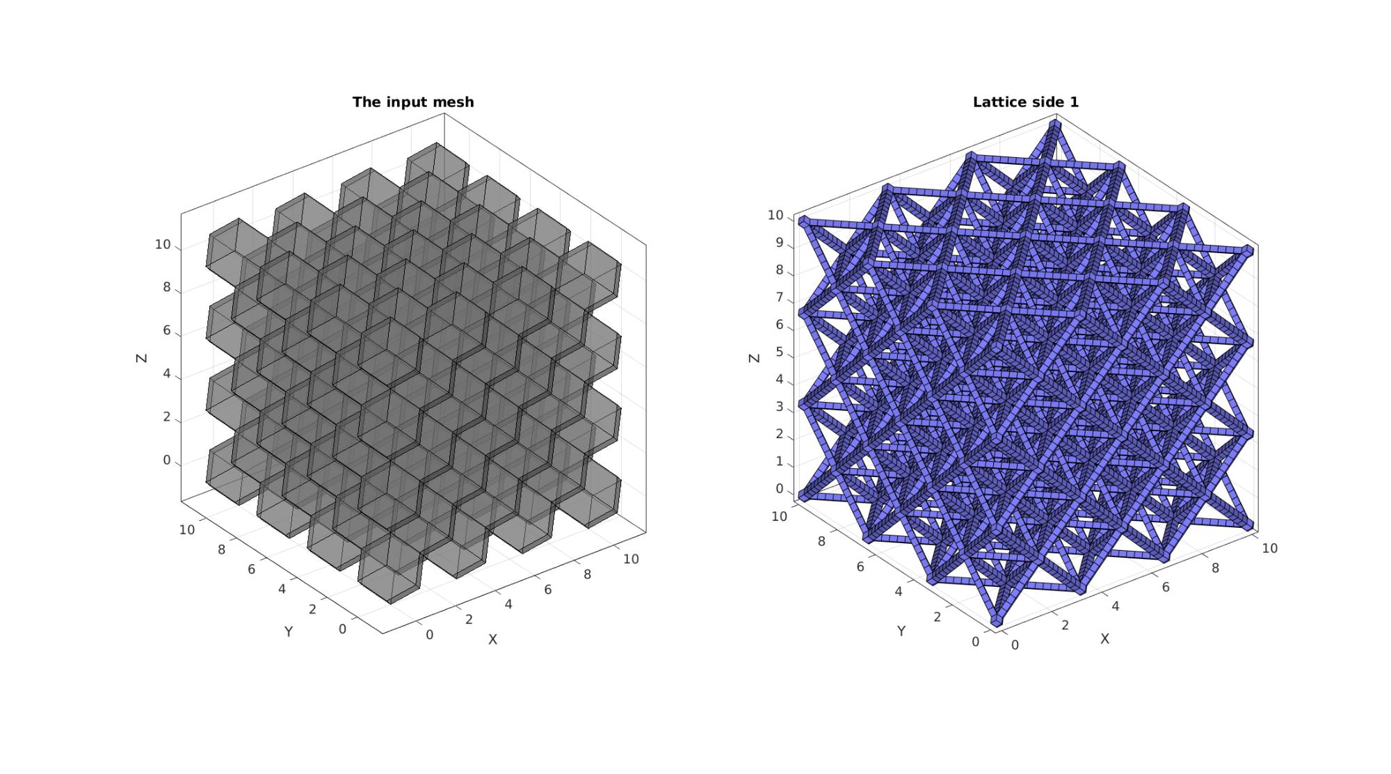
Visualizing input mesh and lattic structures

cFigure;
hs=subplot(1,2,1);
title('The input mesh','fontSize',fontSize)
hold on;
gpatch(Fr,Vr,0.5*ones(1,3),'k',0.5);
axisGeom(gca,fontSize);
camlight headlight; lighting flat;

subplot(1,2,2);
title('Lattice side 1','fontSize',fontSize)
hold on;
gpatch(Fb,V,'bw','k',1);
% patchNormPlot(Fs,Vs);
axisGeom(gca,fontSize);
camlight headlight; lighting flat;

drawnow;

DEFINE BC's

% Define node set logics
indAll=(1:1:size(V,1))';
logicBoundary=ismember(indAll,Fb);

Z=V(:,3);
logicTop=Z>=(sampleSize-eps(sampleSize))& logicBoundary;
logicBottom=Z<=eps(sampleSize) & logicBoundary;

X=V(:,1);
logicSide1=X>=(sampleSize-eps(sampleSize))& logicBoundary;
logicSide2=X<=eps(sampleSize)& logicBoundary;

Y=V(:,2);
logicSide3=Y>=(sampleSize-eps(sampleSize))& logicBoundary;
logicSide4=Y<=eps(sampleSize)& logicBoundary;

%Prescribed force nodes
bcPrescribeListCell{1}=find(logicSide1)';
bcPrescribeListCell{2}=find(logicSide2)';
bcPrescribeListCell{3}=find(logicSide3)';
bcPrescribeListCell{4}=find(logicSide4)';
bcPrescribeListCell{5}=find(logicTop)';
bcPrescribeListCell{6}=find(logicBottom)';

Smoothing lattice

% indKeep=unique([bcPrescribeListCell{:}]);
% [Fb_clean,Vb_clean,indFix]=patchCleanUnused(Fb,Vs);
%
% cPar.Method='HC';
% cPar.n=6;
%
% cPar.RigidConstraints=indFix(indKeep);
% % cPar.RigidConstraints=cPar.RigidConstraints(cPar.RigidConstraints>0);
%
% [Vb_clean]=tesSmooth(Fb_clean,Vb_clean,[],cPar);
% ind=Fb(:);
% ind=unique(ind(:));
% Vs(ind,:)=Vb_clean;

% cFigure; hold on;
% gpatch(Fb,Vs,'bw','k',1);
% % patchNormPlot(Fs,Vs);
% % plotV(Vs(indKeep,:),'k.','MarkerSize',25)
% axisGeom(gca,fontSize);
% camlight headlight; lighting flat;
% drawnow;

Visualizing input mesh and lattic structures

cFigure;
hs=subplot(1,2,1);
title('The input mesh','fontSize',fontSize)
hold on;
gpatch(Fr,Vr,0.5*ones(1,3),'k',0.5);
axisGeom(gca,fontSize);
camlight headlight; lighting flat;

subplot(1,2,2);
title('Lattice side 1','fontSize',fontSize)
hold on;
gpatch(Fb,V,'bw');
% patchNormPlot(Fs,Vs);
axisGeom(gca,fontSize);
camlight headlight; lighting flat;

drawnow;

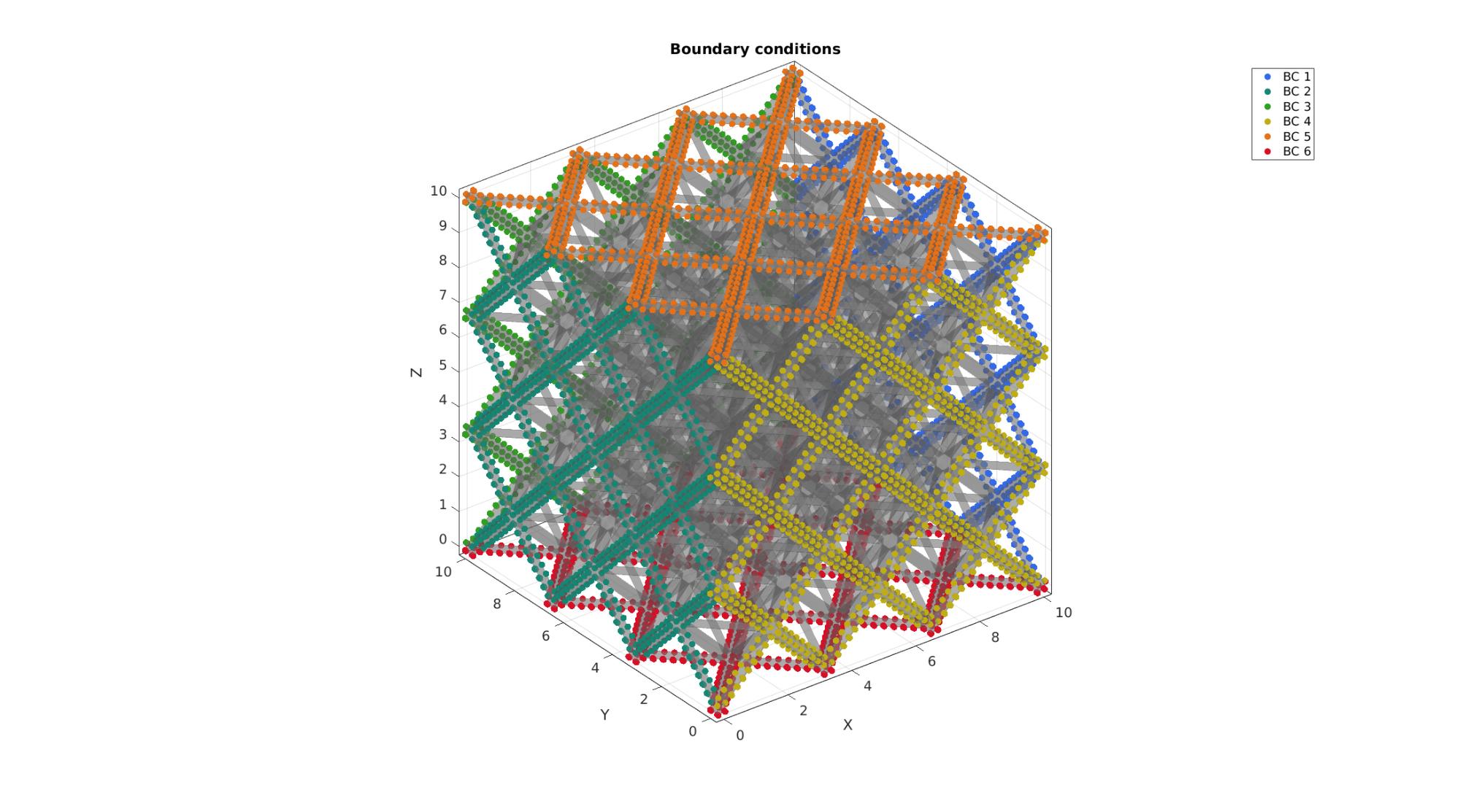
Visualize BC's

cFigure; hold on;
title('Boundary conditions','FontSize',fontSize);
gpatch(Fb,V,'kw','none',0.4);
hl=gobjects(1,6);
plotColors=gjet(6);
for q=1:1:numel(bcPrescribeListCell)
    hl(q)=plotV(V(bcPrescribeListCell{q},:),'k.','MarkerSize',markerSize);
    hl(q).Color=plotColors(q,:);
end

legend(hl,{'BC 1','BC 2','BC 3','BC 4','BC 5','BC 6'});
axisGeom;
camlight headlight;
set(gca,'FontSize',fontSize);
drawnow;

Defining the FEBio input structure

See also febioStructTemplate and febioStruct2xml and the FEBio user manual.

%Get a template with default settings
[febio_spec]=febioStructTemplate;

%febio_spec version
febio_spec.ATTR.version='4.0';

%Module section
febio_spec.Module.ATTR.type='solid';

%Control section
febio_spec.Control.analysis='STATIC';
febio_spec.Control.time_steps=numTimeSteps;
febio_spec.Control.step_size=1/numTimeSteps;
febio_spec.Control.solver.max_refs=max_refs;
febio_spec.Control.solver.qn_method.max_ups=max_ups;
febio_spec.Control.time_stepper.dtmin=dtmin;
febio_spec.Control.time_stepper.dtmax=dtmax;
febio_spec.Control.time_stepper.max_retries=max_retries;
febio_spec.Control.time_stepper.opt_iter=opt_iter;

%Material section
materialName1='Material1';
febio_spec.Material.material{1}.ATTR.name=materialName1;
febio_spec.Material.material{1}.ATTR.type='Ogden';
febio_spec.Material.material{1}.ATTR.id=1;
febio_spec.Material.material{1}.c1=c1;
febio_spec.Material.material{1}.m1=m1;
% febio_spec.Material.material{1}.c2=c1;
% febio_spec.Material.material{1}.m2=-m1;
febio_spec.Material.material{1}.k=k;


% Mesh section
% -> Nodes
febio_spec.Mesh.Nodes{1}.ATTR.name='Object1_lattice'; %The node set name
febio_spec.Mesh.Nodes{1}.node.ATTR.id=(1:size(V,1))'; %The node id's
febio_spec.Mesh.Nodes{1}.node.VAL=V; %The nodel coordinates

% -> Elements
partName1='Part1_lattice';
febio_spec.Mesh.Elements{1}.ATTR.name=partName1; %Name of this part
febio_spec.Mesh.Elements{1}.ATTR.type='hex8'; %Element type
febio_spec.Mesh.Elements{1}.elem.ATTR.id=(1:1:size(E,1))'; %Element id's
febio_spec.Mesh.Elements{1}.elem.VAL=E; %The element matrix

% -> NodeSets
for q=1:1:numel(bcPrescribeListCell)
    febio_spec.Mesh.NodeSet{q}.ATTR.name=['bcPrescribeList_',num2str(q)];
    febio_spec.Mesh.NodeSet{q}.VAL=mrow(bcPrescribeListCell{q});
end

%MeshDomains section
febio_spec.MeshDomains.SolidDomain.ATTR.name=partName1;
febio_spec.MeshDomains.SolidDomain.ATTR.mat=materialName1;

%Boundary condition section

% -> Prescribe boundary conditions
directionStringSet={'x','x','y','y','z','z'};
displacementMagnitudeDir=[1 -1 1 -1 1 -1];
for q=1:1:numel(bcPrescribeListCell)
    nodeSetName=febio_spec.Mesh.NodeSet{q}.ATTR.name;
    febio_spec.Boundary.bc{q}.ATTR.name=['prescibed_displacement_',directionStringSet{q}];
    febio_spec.Boundary.bc{q}.ATTR.type='prescribed displacement';
    febio_spec.Boundary.bc{q}.ATTR.node_set=nodeSetName;
    febio_spec.Boundary.bc{q}.dof=directionStringSet{q};
    febio_spec.Boundary.bc{q}.value.ATTR.lc=1;
    febio_spec.Boundary.bc{q}.value.VAL=displacementMagnitudeDir(q).*displacementMagnitude;
    febio_spec.Boundary.bc{q}.relative=0;
end

%LoadData section
% -> load_controller
febio_spec.LoadData.load_controller{1}.ATTR.name='LC_1';
febio_spec.LoadData.load_controller{1}.ATTR.id=1;
febio_spec.LoadData.load_controller{1}.ATTR.type='loadcurve';
febio_spec.LoadData.load_controller{1}.interpolate='LINEAR';
%febio_spec.LoadData.load_controller{1}.extend='CONSTANT';
febio_spec.LoadData.load_controller{1}.points.pt.VAL=[0 0; 1 1];

%Output section
% -> log file
febio_spec.Output.logfile.ATTR.file=febioLogFileName;

febio_spec.Output.logfile.node_data{1}.ATTR.file=febioLogFileName_disp;
febio_spec.Output.logfile.node_data{1}.ATTR.data='ux;uy;uz';
febio_spec.Output.logfile.node_data{1}.ATTR.delim=',';

febio_spec.Output.logfile.node_data{2}.ATTR.file=febioLogFileName_force;
febio_spec.Output.logfile.node_data{2}.ATTR.data='Rx;Ry;Rz';
febio_spec.Output.logfile.node_data{2}.ATTR.delim=',';

febio_spec.Output.logfile.element_data{1}.ATTR.file=febioLogFileName_stress;
febio_spec.Output.logfile.element_data{1}.ATTR.data='sz';
febio_spec.Output.logfile.element_data{1}.ATTR.delim=',';

% Plotfile section
febio_spec.Output.plotfile.compression=0;

Quick viewing of the FEBio input file structure

The febView function can be used to view the xml structure in a MATLAB figure window.

febView(febio_spec); %Viewing the febio file

Exporting the FEBio input file

Exporting the febio_spec structure to an FEBio input file is done using the febioStruct2xml function.

febioStruct2xml(febio_spec,febioFebFileName); %Exporting to file and domNode
%system(['gedit ',febioFebFileName,' &']);

Running the FEBio analysis

To run the analysis defined by the created FEBio input file the runMonitorFEBio function is used. The input for this function is a structure defining job settings e.g. the FEBio input file name. The optional output runFlag informs the user if the analysis was run succesfully.

febioAnalysis.run_filename=febioFebFileName; %The input file name
febioAnalysis.run_logname=febioLogFileName; %The name for the log file
febioAnalysis.disp_on=1; %Display information on the command window
febioAnalysis.runMode=runMode;
febioAnalysis.maxLogCheckTime=10; %Max log file checking time

[runFlag]=runMonitorFEBio(febioAnalysis);%START FEBio NOW!!!!!!!!

 
%%%%%%%%%%%%%%%%%%%%%%%%%%%%%%%%%%%%%%%%%%%%%%%%%%%%%%%%%%%%%%%%%%%%%%%%%%%
-------->    RUNNING/MONITORING FEBIO JOB    <-------- 21-Apr-2023 11:44:07
FEBio path: /home/kevin/FEBioStudio2/bin/febio4
# Attempt removal of existing log files                21-Apr-2023 11:44:07
 * Removal succesful                                   21-Apr-2023 11:44:07
# Attempt removal of existing .xplt files              21-Apr-2023 11:44:07
 * Removal succesful                                   21-Apr-2023 11:44:07
# Starting FEBio...                                    21-Apr-2023 11:44:07
  Max. total analysis time is: Inf s
 * Waiting for log file creation                       21-Apr-2023 11:44:07
   Max. wait time: 10 s
 * Log file found.                                     21-Apr-2023 11:44:07
# Parsing log file...                                  21-Apr-2023 11:44:07
    number of iterations   : 2                         21-Apr-2023 11:44:08
    number of reformations : 2                         21-Apr-2023 11:44:08
------- converged at time : 0.04                       21-Apr-2023 11:44:08
    number of iterations   : 32                        21-Apr-2023 11:44:19
    number of reformations : 32                        21-Apr-2023 11:44:19
------- converged at time : 0.08                       21-Apr-2023 11:44:19
    number of iterations   : 11                        21-Apr-2023 11:44:23
    number of reformations : 11                        21-Apr-2023 11:44:23
------- converged at time : 0.0975473                  21-Apr-2023 11:44:23
    number of iterations   : 11                        21-Apr-2023 11:44:27
    number of reformations : 11                        21-Apr-2023 11:44:27
------- converged at time : 0.110611                   21-Apr-2023 11:44:27
    number of iterations   : 8                         21-Apr-2023 11:44:31
    number of reformations : 8                         21-Apr-2023 11:44:31
------- converged at time : 0.118739                   21-Apr-2023 11:44:31
    number of iterations   : 6                         21-Apr-2023 11:44:34
    number of reformations : 6                         21-Apr-2023 11:44:34
------- converged at time : 0.125831                   21-Apr-2023 11:44:34
    number of iterations   : 5                         21-Apr-2023 11:44:35
    number of reformations : 5                         21-Apr-2023 11:44:35
------- converged at time : 0.132924                   21-Apr-2023 11:44:35
    number of iterations   : 4                         21-Apr-2023 11:44:37
    number of reformations : 4                         21-Apr-2023 11:44:37
------- converged at time : 0.143157                   21-Apr-2023 11:44:37
    number of iterations   : 4                         21-Apr-2023 11:44:38
    number of reformations : 4                         21-Apr-2023 11:44:38
------- converged at time : 0.159343                   21-Apr-2023 11:44:38
    number of iterations   : 4                         21-Apr-2023 11:44:40
    number of reformations : 4                         21-Apr-2023 11:44:40
------- converged at time : 0.180292                   21-Apr-2023 11:44:40
    number of iterations   : 4                         21-Apr-2023 11:44:42
    number of reformations : 4                         21-Apr-2023 11:44:42
------- converged at time : 0.205052                   21-Apr-2023 11:44:42
    number of iterations   : 8                         21-Apr-2023 11:44:45
    number of reformations : 8                         21-Apr-2023 11:44:45
------- converged at time : 0.232859                   21-Apr-2023 11:44:45
    number of iterations   : 6                         21-Apr-2023 11:44:47
    number of reformations : 6                         21-Apr-2023 11:44:47
------- converged at time : 0.256995                   21-Apr-2023 11:44:47
    number of iterations   : 5                         21-Apr-2023 11:44:49
    number of reformations : 5                         21-Apr-2023 11:44:49
------- converged at time : 0.28113                    21-Apr-2023 11:44:49
    number of iterations   : 9                         21-Apr-2023 11:44:52
    number of reformations : 9                         21-Apr-2023 11:44:52
------- converged at time : 0.30678                    21-Apr-2023 11:44:52
    number of iterations   : 4                         21-Apr-2023 11:44:54
    number of reformations : 4                         21-Apr-2023 11:44:54
------- converged at time : 0.327797                   21-Apr-2023 11:44:54
    number of iterations   : 4                         21-Apr-2023 11:44:55
    number of reformations : 4                         21-Apr-2023 11:44:55
------- converged at time : 0.35261                    21-Apr-2023 11:44:55
    number of iterations   : 4                         21-Apr-2023 11:44:57
    number of reformations : 4                         21-Apr-2023 11:44:57
------- converged at time : 0.38046                    21-Apr-2023 11:44:57
    number of iterations   : 4                         21-Apr-2023 11:44:58
    number of reformations : 4                         21-Apr-2023 11:44:58
------- converged at time : 0.41074                    21-Apr-2023 11:44:58
    number of iterations   : 4                         21-Apr-2023 11:45:00
    number of reformations : 4                         21-Apr-2023 11:45:00
------- converged at time : 0.442965                   21-Apr-2023 11:45:00
    number of iterations   : 4                         21-Apr-2023 11:45:02
    number of reformations : 4                         21-Apr-2023 11:45:02
------- converged at time : 0.476744                   21-Apr-2023 11:45:02
    number of iterations   : 4                         21-Apr-2023 11:45:03
    number of reformations : 4                         21-Apr-2023 11:45:03
------- converged at time : 0.511768                   21-Apr-2023 11:45:03
    number of iterations   : 4                         21-Apr-2023 11:45:05
    number of reformations : 4                         21-Apr-2023 11:45:05
------- converged at time : 0.547787                   21-Apr-2023 11:45:05
    number of iterations   : 4                         21-Apr-2023 11:45:07
    number of reformations : 4                         21-Apr-2023 11:45:07
------- converged at time : 0.584602                   21-Apr-2023 11:45:07
    number of iterations   : 4                         21-Apr-2023 11:45:08
    number of reformations : 4                         21-Apr-2023 11:45:08
------- converged at time : 0.622054                   21-Apr-2023 11:45:08
    number of iterations   : 4                         21-Apr-2023 11:45:10
    number of reformations : 4                         21-Apr-2023 11:45:10
------- converged at time : 0.660015                   21-Apr-2023 11:45:10
    number of iterations   : 4                         21-Apr-2023 11:45:11
    number of reformations : 4                         21-Apr-2023 11:45:11
------- converged at time : 0.698385                   21-Apr-2023 11:45:11
    number of iterations   : 4                         21-Apr-2023 11:45:13
    number of reformations : 4                         21-Apr-2023 11:45:13
------- converged at time : 0.73708                    21-Apr-2023 11:45:13
    number of reformations : 4                         21-Apr-2023 11:45:15
------- converged at time : 0.776037                   21-Apr-2023 11:45:15
    number of iterations   : 4                         21-Apr-2023 11:45:16
    number of reformations : 4                         21-Apr-2023 11:45:16
------- converged at time : 0.815202                   21-Apr-2023 11:45:16
    number of iterations   : 4                         21-Apr-2023 11:45:18
    number of reformations : 4                         21-Apr-2023 11:45:18
------- converged at time : 0.854534                   21-Apr-2023 11:45:18
    number of iterations   : 4                         21-Apr-2023 11:45:19
    number of reformations : 4                         21-Apr-2023 11:45:19
------- converged at time : 0.893999                   21-Apr-2023 11:45:19
    number of iterations   : 4                         21-Apr-2023 11:45:21
    number of reformations : 4                         21-Apr-2023 11:45:21
------- converged at time : 0.933572                   21-Apr-2023 11:45:21
    number of iterations   : 4                         21-Apr-2023 11:45:22
    number of reformations : 4                         21-Apr-2023 11:45:22
------- converged at time : 0.97323                    21-Apr-2023 11:45:22
    number of iterations   : 3                         21-Apr-2023 11:45:24
    number of reformations : 3                         21-Apr-2023 11:45:24
------- converged at time : 1                          21-Apr-2023 11:45:24
 Elapsed time : 0:01:17                                21-Apr-2023 11:45:24
 N O R M A L   T E R M I N A T I O N
# Done                                                 21-Apr-2023 11:45:24
%%%%%%%%%%%%%%%%%%%%%%%%%%%%%%%%%%%%%%%%%%%%%%%%%%%%%%%%%%%%%%%%%%%%%%%%%%%

Import FEBio results

if runFlag==1 %i.e. a succesful run

    % Importing nodal displacements from a log file
    dataStruct=importFEBio_logfile(fullfile(savePath,febioLogFileName_disp),0,1);

    %Access data
    N_disp_mat=dataStruct.data; %Displacement
    timeVec=dataStruct.time; %Time

    %Create deformed coordinate set
    V_DEF=N_disp_mat+repmat(V,[1 1 size(N_disp_mat,3)]);

    % Importing nodal forces
    dataStruct=importFEBio_logfile(fullfile(savePath,febioLogFileName_force),0,1);
    N_force_mat=dataStruct.data;

    indicesSide=bcPrescribeListCell{1};
    areaSide=sampleSize.^2;

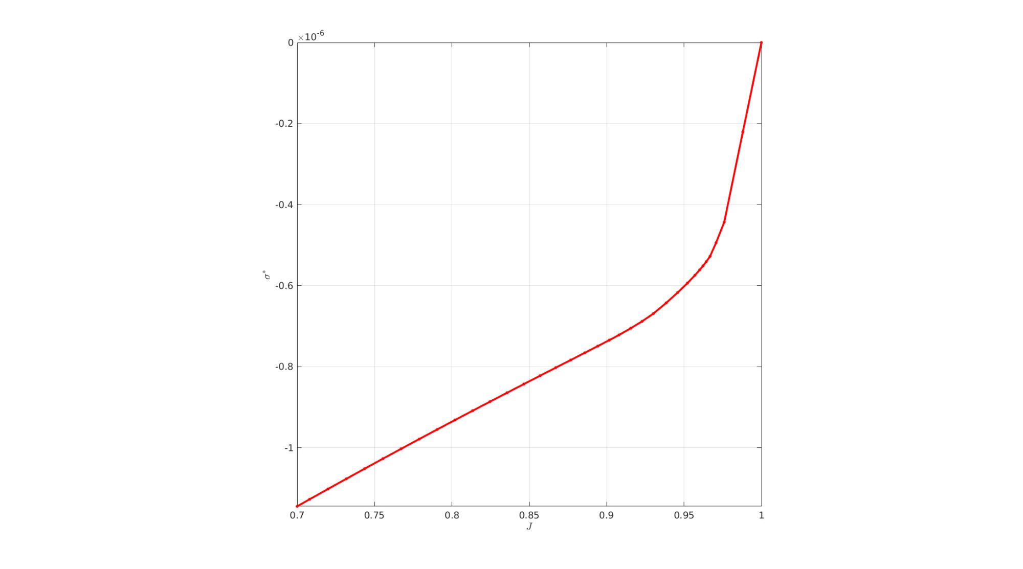
    stressVal=mean(squeeze(N_force_mat(indicesSide,1,:))./areaSide,1);
    J_Val=1-((1-J_final).*timeVec(:));

    cFigure; hold on;
    xlabel('$J$','Interpreter','Latex'); ylabel('$\sigma^*$','Interpreter','Latex');
    plot(J_Val(:),stressVal(:),'r.-','LineWidth',3,'MarkerSize',15);
    axis square; axis tight; grid on; box on;
    set(gca,'FontSize',fontSize);
    drawnow;

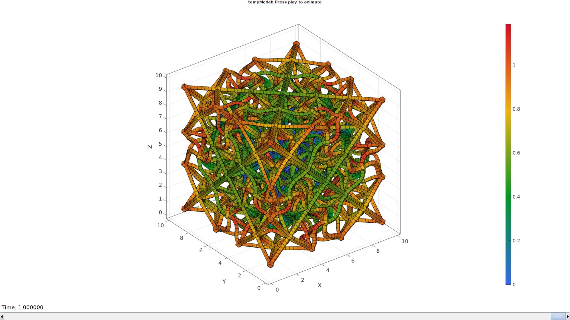
Plotting the simulated results using anim8 to visualize and animate deformations

    DN_magnitude=sqrt(sum(N_disp_mat(:,:,end).^2,2)); %Current displacement magnitude

    % Create basic view and store graphics handle to initiate animation
    hf=cFigure; %Open figure
    gtitle([febioFebFileNamePart,': Press play to animate']);
    hp=gpatch(Fb,V_DEF(:,:,end),DN_magnitude,'k',1); %Add graphics object to animate
    %     gpatch(Fb,Vs,'kw','none',0.25); %A static graphics object
    hp.FaceColor='interp';

    axisGeom(gca,fontSize);
    colormap(gjet(250)); colorbar;
    caxis([0 max(DN_magnitude)]);
    axis(axisLim(V_DEF)); %Set axis limits statically
    %     view(130,25); %Set view direction
    camlight headlight;

    % Set up animation features
    animStruct.Time=timeVec; %The time vector
    for qt=1:1:size(N_disp_mat,3) %Loop over time increments
        DN=N_disp_mat(:,:,qt); %Current displacement
        DN_magnitude=sqrt(sum(DN.^2,2)); %Current displacement magnitude

        %Set entries in animation structure
        animStruct.Handles{qt}=[hp hp]; %Handles of objects to animate
        animStruct.Props{qt}={'Vertices','CData'}; %Properties of objects to animate
        animStruct.Set{qt}={V_DEF(:,:,qt),DN_magnitude}; %Property values for to set in order to animate
    end
    anim8(hf,animStruct); %Initiate animation feature
    drawnow;

end

GIBBON www.gibboncode.org

Kevin Mattheus Moerman, [email protected]

GIBBON footer text

License: https://github.com/gibbonCode/GIBBON/blob/master/LICENSE

GIBBON: The Geometry and Image-based Bioengineering add-On. A toolbox for image segmentation, image-based modeling, meshing, and finite element analysis.

This program is free software: you can redistribute it and/or modify it under the terms of the GNU General Public License as published by the Free Software Foundation, either version 3 of the License, or (at your option) any later version.

This program is distributed in the hope that it will be useful, but WITHOUT ANY WARRANTY; without even the implied warranty of MERCHANTABILITY or FITNESS FOR A PARTICULAR PURPOSE. See the GNU General Public License for more details.

You should have received a copy of the GNU General Public License along with this program. If not, see http://www.gnu.org/licenses/.