DEMO_febio_0019_vessel_pressure_inflate

Below is a demonstration for:

Building geometry for a cylindrical vessel with tetrahedral elements
Defining the boundary conditions
Coding the febio structure
Running the model
Importing and visualizing the displacement results

Keywords
Plot settings
Control parameters
Creating model boundary polygons
Creating model boundary surfaces
Defining the boundary conditions
Defining the FEBio input structure
Quick viewing of the FEBio input file structure
Exporting the FEBio input file
Running the FEBio analysis
Import FEBio results

Keywords

febio_spec version 4.0
febio, FEBio
vessel, cylinder
prescribed pressure
tetrahedral elements, tet4
tube, cylindrical
static, solid
hyperelastic, Ogden
displacement logfile
stress logfile

clear; close all; clc;

Plot settings

fontSize=20;
faceAlpha1=0.8;
markerSize=40;
markerSize2=20;
lineWidth=3;

Control parameters

% Path names
defaultFolder = fileparts(fileparts(mfilename('fullpath')));
savePath=fullfile(defaultFolder,'data','temp');

% Defining file names
febioFebFileNamePart='tempModel';
febioFebFileName=fullfile(savePath,[febioFebFileNamePart,'.feb']); %FEB file name
febioLogFileName=[febioFebFileNamePart,'.txt']; %FEBio log file name
febioLogFileName_disp=[febioFebFileNamePart,'_disp_out.txt']; %Log file name for exporting displacement
febioLogFileName_stress_prin=[febioFebFileNamePart,'_stress_prin_out.txt']; %Log file name for exporting principal stress

%Specifying geometry parameters
pointSpacing=1;

radiusInner1=9;
radiusInner2=10;

radiusOuter1=10;
radiusOuter2=12;

vesselLength=50;

%Load
appliedPressure=0.1; %MPa

%Material parameter set
c1=1; %Shear-modulus-like parameter
m1=2; %Material parameter setting degree of non-linearity
k_factor=1e2; %Bulk modulus factor
k=c1*k_factor; %Bulk modulus

% FEA control settings
numTimeSteps=10; %Number of time steps desired
max_refs=25; %Max reforms
max_ups=0; %Set to zero to use full-Newton iterations
opt_iter=6; %Optimum number of iterations
max_retries=5; %Maximum number of retires
dtmin=(1/numTimeSteps)/100; %Minimum time step size
dtmax=1/numTimeSteps; %Maximum time step size

runMode='external';% 'internal' or 'external'

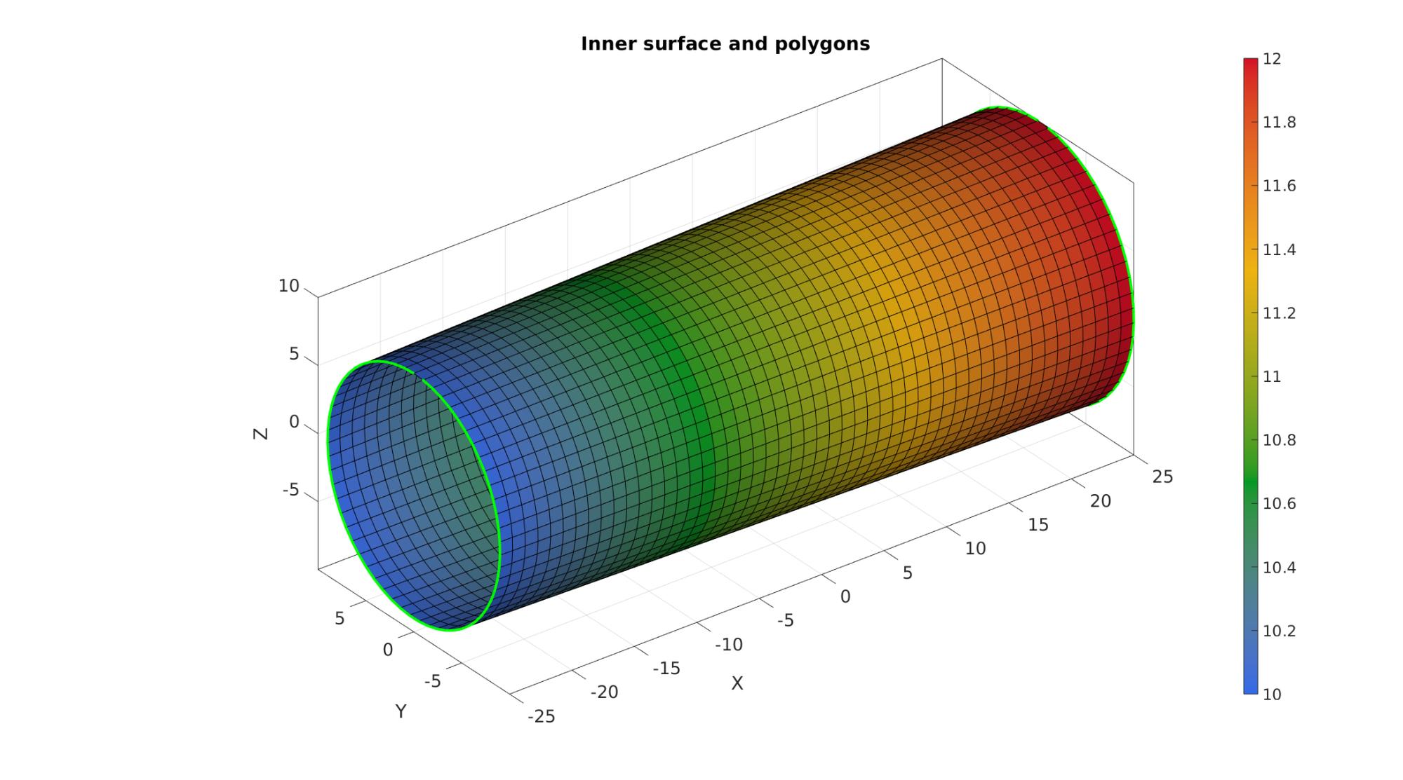
Creating model boundary polygons

nRad=round((2*pi*mean([radiusInner1 radiusInner2]))/pointSpacing); %Number of radial steps

t=linspace(0,2*pi,nRad)'; %Angles
t=t(1:end-1); %take away last which equals start
v1_Inner=[-(vesselLength/2)*ones(size(t)) radiusInner1*sin(t) radiusInner1*cos(t)]; %Circular coordinates

t=linspace(0,2*pi,nRad)'; %Angles
t=t(1:end-1); %take away last which equals start
v2_Inner=[(vesselLength/2)*ones(size(t)) radiusInner2*sin(t) radiusInner2*cos(t)]; %Circular coordinates

Creating model boundary surfaces

% controlStructLoft.numSteps=17;
controlStructLoft.closeLoopOpt=1;
controlStructLoft.patchType='quad';

%Meshing outer surface
[F1,V1]=polyLoftLinear(v1_Inner,v2_Inner,controlStructLoft);
F1=fliplr(F1); %Invert orientation

outerRadii=V1(:,1); %x
outerRadii=outerRadii-min(outerRadii(:)); %[0 - ...]
outerRadii=outerRadii./max(outerRadii(:)); %[0 - 1]
outerRadii=radiusOuter1+(outerRadii.*(radiusOuter2-radiusOuter1)); %[0 - 1]

innerRadii=V1(:,1); %x
innerRadii=innerRadii-min(innerRadii(:)); %[0 - ...]
innerRadii=innerRadii./max(innerRadii(:)); %[0 - 1]
innerRadii=radiusInner1+(innerRadii.*(radiusInner2-radiusInner1)); %[0 - 1]

wallThickness=outerRadii-innerRadii;

Plotting model boundary polygons

cFigure; hold on;
title('Inner surface and polygons','FontSize',fontSize);
gpatch(F1,V1,outerRadii);
plotV(v1_Inner,'g.-','LineWidth',3);
plotV(v2_Inner,'g.-','LineWidth',3);
axisGeom(gca,fontSize); camlight headlight;
colormap gjet; colorbar;
gdrawnow;

numSteps=ceil(max(wallThickness)./pointSpacing);
[E,V,Fp1,Fp2]=patchThick(F1,V1,1,wallThickness,numSteps);

[F,~,C_type]=element2patch(E,[],'hex8');
indBoundary=tesBoundary(F);
Fb=F(indBoundary,:);
Cb=C_type(indBoundary,:);

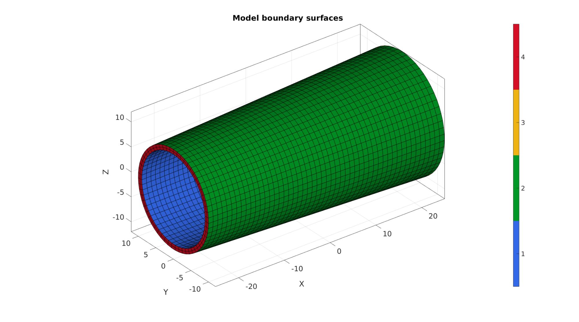
Plotting model boundary surfaces

cFigure;
hold on;
title('Model boundary surfaces','FontSize',fontSize);

gpatch(Fb,V,Cb);

axisGeom(gca,fontSize); camlight headlight;
colormap gjet; icolorbar;
drawnow;

Defining the boundary conditions

The visualization of the model boundary shows colors for each side of the cube. These labels can be used to define boundary conditions.

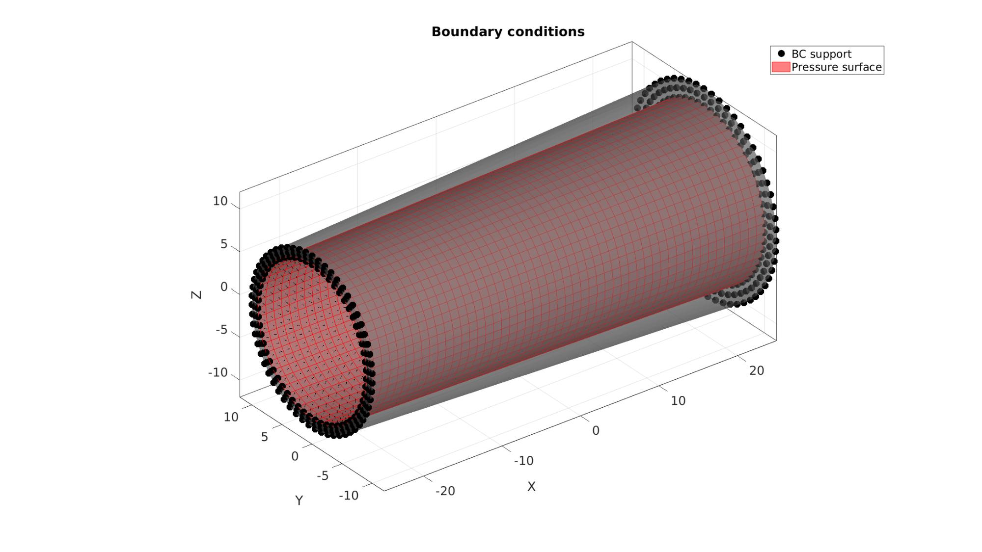
%Define supported node set
bcSupportList=unique(Fb(ismember(Cb,[3 4]),:)); %Node set part of selected face

F_pressure=Fb(Cb==1,:);

Visualizing boundary conditions. Markers plotted on the semi-transparent model denote the nodes in the various boundary condition lists.

hf=cFigure;
title('Boundary conditions','FontSize',fontSize);
xlabel('X','FontSize',fontSize); ylabel('Y','FontSize',fontSize); zlabel('Z','FontSize',fontSize);
hold on;

gpatch(Fb,V,'kw','none',0.5);

hl(1)=plotV(V(bcSupportList,:),'k.','MarkerSize',markerSize);
hl(2)=gpatch(F_pressure,V,'rw','r',1);
patchNormPlot(F_pressure,V);

legend(hl,{'BC support','Pressure surface'});

axisGeom(gca,fontSize);
camlight headlight;
drawnow;

Defining the FEBio input structure

See also febioStructTemplate and febioStruct2xml and the FEBio user manual.

%Get a template with default settings
[febio_spec]=febioStructTemplate;

%febio_spec version
febio_spec.ATTR.version='4.0';

%Module section
febio_spec.Module.ATTR.type='solid';

%Control section
febio_spec.Control.analysis='STATIC';
febio_spec.Control.time_steps=numTimeSteps;
febio_spec.Control.step_size=1/numTimeSteps;
febio_spec.Control.solver.max_refs=max_refs;
febio_spec.Control.solver.qn_method.max_ups=max_ups;
febio_spec.Control.time_stepper.dtmin=dtmin;
febio_spec.Control.time_stepper.dtmax=dtmax;
febio_spec.Control.time_stepper.max_retries=max_retries;
febio_spec.Control.time_stepper.opt_iter=opt_iter;

%Material section
materialName1='Material1';
febio_spec.Material.material{1}.ATTR.name=materialName1;
febio_spec.Material.material{1}.ATTR.type='Ogden';
febio_spec.Material.material{1}.ATTR.id=1;
febio_spec.Material.material{1}.c1=c1;
febio_spec.Material.material{1}.m1=m1;
febio_spec.Material.material{1}.c2=c1;
febio_spec.Material.material{1}.m2=-m1;
febio_spec.Material.material{1}.k=k;

%Mesh section
% -> Nodes
febio_spec.Mesh.Nodes{1}.ATTR.name='nodeSet_all'; %The node set name
febio_spec.Mesh.Nodes{1}.node.ATTR.id=(1:size(V,1))'; %The node id's
febio_spec.Mesh.Nodes{1}.node.VAL=V; %The nodel coordinates

% -> Elements
partName1='Part1';
febio_spec.Mesh.Elements{1}.ATTR.name=partName1; %Name of this part
febio_spec.Mesh.Elements{1}.ATTR.type='hex8'; %Element type
febio_spec.Mesh.Elements{1}.elem.ATTR.id=(1:1:size(E,1))'; %Element id's
febio_spec.Mesh.Elements{1}.elem.VAL=E; %The element matrix

% -> Surfaces
surfaceName1='LoadedSurface';
febio_spec.Mesh.Surface{1}.ATTR.name=surfaceName1;
febio_spec.Mesh.Surface{1}.quad4.ATTR.id=(1:1:size(F_pressure,1))';
febio_spec.Mesh.Surface{1}.quad4.VAL=F_pressure;

% -> NodeSets
nodeSetName1='bcSupportList';
febio_spec.Mesh.NodeSet{1}.ATTR.name=nodeSetName1;
febio_spec.Mesh.NodeSet{1}.VAL=mrow(bcSupportList);

%MeshDomains section
febio_spec.MeshDomains.SolidDomain.ATTR.name=partName1;
febio_spec.MeshDomains.SolidDomain.ATTR.mat=materialName1;

%Boundary condition section
% -> Fix boundary conditions
febio_spec.Boundary.bc{1}.ATTR.name='zero_displacement_xyz';
febio_spec.Boundary.bc{1}.ATTR.type='zero displacement';
febio_spec.Boundary.bc{1}.ATTR.node_set=nodeSetName1;
febio_spec.Boundary.bc{1}.x_dof=1;
febio_spec.Boundary.bc{1}.y_dof=1;
febio_spec.Boundary.bc{1}.z_dof=1;

%Loads section
% -> Surface load
febio_spec.Loads.surface_load{1}.ATTR.type='pressure';
febio_spec.Loads.surface_load{1}.ATTR.surface=surfaceName1;
febio_spec.Loads.surface_load{1}.pressure.ATTR.lc=1;
febio_spec.Loads.surface_load{1}.pressure.VAL=appliedPressure;
febio_spec.Loads.surface_load{1}.symmetric_stiffness=1;

%LoadData section
% -> load_controller
febio_spec.LoadData.load_controller{1}.ATTR.name='LC_1';
febio_spec.LoadData.load_controller{1}.ATTR.id=1;
febio_spec.LoadData.load_controller{1}.ATTR.type='loadcurve';
febio_spec.LoadData.load_controller{1}.interpolate='LINEAR';
%febio_spec.LoadData.load_controller{1}.extend='CONSTANT';
febio_spec.LoadData.load_controller{1}.points.pt.VAL=[0 0; 1 1];

%Output section
% -> log file
febio_spec.Output.logfile.ATTR.file=febioLogFileName;
febio_spec.Output.logfile.node_data{1}.ATTR.file=febioLogFileName_disp;
febio_spec.Output.logfile.node_data{1}.ATTR.data='ux;uy;uz';
febio_spec.Output.logfile.node_data{1}.ATTR.delim=',';

febio_spec.Output.logfile.element_data{1}.ATTR.file=febioLogFileName_stress_prin;
febio_spec.Output.logfile.element_data{1}.ATTR.data='s1;s2;s3';
febio_spec.Output.logfile.element_data{1}.ATTR.delim=',';

febio_spec.Output.plotfile.compression=0;

Quick viewing of the FEBio input file structure

The febView function can be used to view the xml structure in a MATLAB figure window.

febView(febio_spec); %Viewing the febio file

Exporting the FEBio input file

Exporting the febio_spec structure to an FEBio input file is done using the febioStruct2xml function.

febioStruct2xml(febio_spec,febioFebFileName); %Exporting to file and domNode
%system(['gedit ',febioFebFileName,' &']);

Running the FEBio analysis

To run the analysis defined by the created FEBio input file the runMonitorFEBio function is used. The input for this function is a structure defining job settings e.g. the FEBio input file name. The optional output runFlag informs the user if the analysis was run succesfully.

febioAnalysis.run_filename=febioFebFileName; %The input file name
febioAnalysis.run_logname=febioLogFileName; %The name for the log file
febioAnalysis.disp_on=1; %Display information on the command window
febioAnalysis.runMode=runMode;
febioAnalysis.maxLogCheckTime=10; %Max log file checking time

[runFlag]=runMonitorFEBio(febioAnalysis);%START FEBio NOW!!!!!!!!

 
%%%%%%%%%%%%%%%%%%%%%%%%%%%%%%%%%%%%%%%%%%%%%%%%%%%%%%%%%%%%%%%%%%%%%%%%%%%
-------->    RUNNING/MONITORING FEBIO JOB    <-------- 24-Jul-2023 10:40:34
FEBio path: /home/kevin/FEBioStudio/bin/febio4
# Attempt removal of existing log files                24-Jul-2023 10:40:34
 * Removal succesful                                   24-Jul-2023 10:40:34
# Attempt removal of existing .xplt files              24-Jul-2023 10:40:34
 * Removal succesful                                   24-Jul-2023 10:40:34
# Starting FEBio...                                    24-Jul-2023 10:40:34
  Max. total analysis time is: Inf s
 * Waiting for log file creation                       24-Jul-2023 10:40:34
   Max. wait time: 10 s
 * Log file found.                                     24-Jul-2023 10:40:34
# Parsing log file...                                  24-Jul-2023 10:40:34
    number of iterations   : 4                         24-Jul-2023 10:40:35
    number of reformations : 4                         24-Jul-2023 10:40:35
------- converged at time : 0.1                        24-Jul-2023 10:40:35
    number of iterations   : 4                         24-Jul-2023 10:40:36
    number of reformations : 4                         24-Jul-2023 10:40:36
------- converged at time : 0.2                        24-Jul-2023 10:40:36
    number of iterations   : 4                         24-Jul-2023 10:40:36
    number of reformations : 4                         24-Jul-2023 10:40:36
------- converged at time : 0.3                        24-Jul-2023 10:40:36
    number of iterations   : 4                         24-Jul-2023 10:40:38
    number of reformations : 4                         24-Jul-2023 10:40:38
------- converged at time : 0.4                        24-Jul-2023 10:40:38
    number of iterations   : 4                         24-Jul-2023 10:40:39
    number of reformations : 4                         24-Jul-2023 10:40:39
------- converged at time : 0.5                        24-Jul-2023 10:40:39
    number of iterations   : 4                         24-Jul-2023 10:40:39
    number of reformations : 4                         24-Jul-2023 10:40:39
------- converged at time : 0.6                        24-Jul-2023 10:40:39
    number of iterations   : 4                         24-Jul-2023 10:40:40
    number of reformations : 4                         24-Jul-2023 10:40:40
------- converged at time : 0.7                        24-Jul-2023 10:40:40
    number of iterations   : 4                         24-Jul-2023 10:40:40
    number of reformations : 4                         24-Jul-2023 10:40:40
------- converged at time : 0.8                        24-Jul-2023 10:40:40
    number of iterations   : 4                         24-Jul-2023 10:40:41
    number of reformations : 4                         24-Jul-2023 10:40:41
------- converged at time : 0.9                        24-Jul-2023 10:40:41
    number of iterations   : 4                         24-Jul-2023 10:40:41
    number of reformations : 4                         24-Jul-2023 10:40:41
------- converged at time : 1                          24-Jul-2023 10:40:41
 Elapsed time : 0:00:07                                24-Jul-2023 10:40:41
 N O R M A L   T E R M I N A T I O N
# Done                                                 24-Jul-2023 10:40:41
%%%%%%%%%%%%%%%%%%%%%%%%%%%%%%%%%%%%%%%%%%%%%%%%%%%%%%%%%%%%%%%%%%%%%%%%%%%

Import FEBio results

if runFlag==1 %i.e. a succesful run

Importing nodal displacements from a log file

    dataStruct=importFEBio_logfile(fullfile(savePath,febioLogFileName_disp),0,1);

    %Access data
    N_disp_mat=dataStruct.data; %Displacement
    timeVec=dataStruct.time; %Time

    %Create deformed coordinate set
    V_DEF=N_disp_mat+repmat(V,[1 1 size(N_disp_mat,3)]);

Importing element principal stresses from a log file

    dataStruct=importFEBio_logfile(fullfile(savePath,febioLogFileName_stress_prin),0,1);

    %Access data
    E_stress_prin_mat=dataStruct.data;
    S1_mat=E_stress_prin_mat(:,1,:);
    S2_mat=E_stress_prin_mat(:,2,:);
    S3_mat=E_stress_prin_mat(:,3,:);
    S_vm = sqrt(((S1_mat-S2_mat).^2+(S2_mat-S3_mat).^2+(S3_mat-S1_mat).^2)./2);

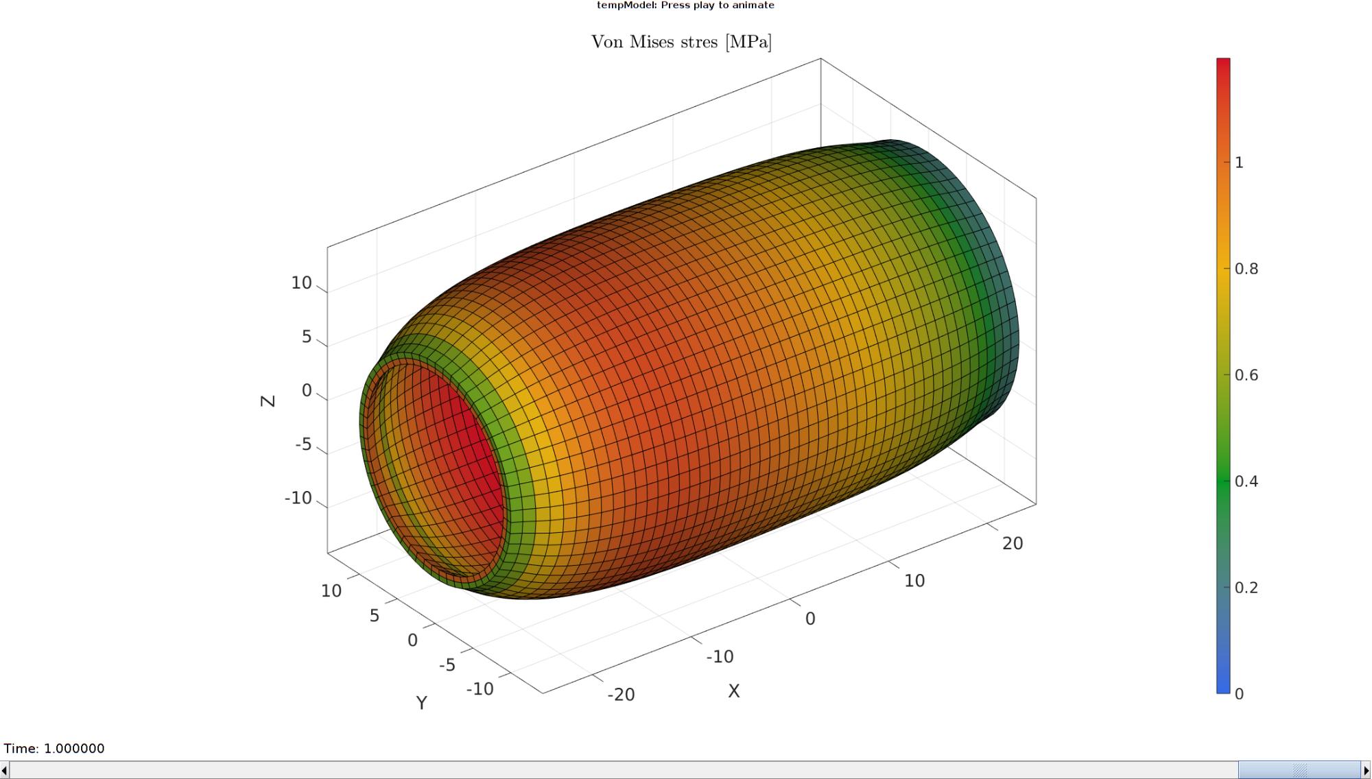
Plotting the simulated results using anim8 to visualize and animate deformations

    [~,CF_S_vm,~]=element2patch(E,S_vm(:,:,end),'hex8');
    Cb_S_vm=CF_S_vm(indBoundary,:);

    % Create basic view and store graphics handle to initiate animation
    hf=cFigure; %Open figure
    gtitle([febioFebFileNamePart,': Press play to animate']);
    title('Von Mises stres [MPa]','Interpreter','Latex')
    hp=gpatch(Fb,V_DEF(:,:,end),Cb_S_vm,'k',1); %Add graphics object to animate

    axisGeom(gca,fontSize);
    colormap(gjet(250)); colorbar;
    caxis([0 max(S_vm(:))]);
    axis(axisLim(V_DEF)); %Set axis limits statically
    camlight headlight;

    % Set up animation features
    animStruct.Time=timeVec; %The time vector
    for qt=1:1:size(N_disp_mat,3) %Loop over time increments
        [~,CF_S_vm,~]=element2patch(E,S_vm(:,:,qt),'hex8');
        Cb_S_vm=CF_S_vm(indBoundary,:);

        %Set entries in animation structure
        animStruct.Handles{qt}=[hp hp]; %Handles of objects to animate
        animStruct.Props{qt}={'Vertices','CData'}; %Properties of objects to animate
        animStruct.Set{qt}={V_DEF(:,:,qt),Cb_S_vm}; %Property values for to set in order to animate
    end
    anim8(hf,animStruct); %Initiate animation feature
    drawnow;

end

GIBBON www.gibboncode.org

Kevin Mattheus Moerman, [email protected]

GIBBON footer text

License: https://github.com/gibbonCode/GIBBON/blob/master/LICENSE

GIBBON: The Geometry and Image-based Bioengineering add-On. A toolbox for image segmentation, image-based modeling, meshing, and finite element analysis.

This program is free software: you can redistribute it and/or modify it under the terms of the GNU General Public License as published by the Free Software Foundation, either version 3 of the License, or (at your option) any later version.

This program is distributed in the hope that it will be useful, but WITHOUT ANY WARRANTY; without even the implied warranty of MERCHANTABILITY or FITNESS FOR A PARTICULAR PURPOSE. See the GNU General Public License for more details.

You should have received a copy of the GNU General Public License along with this program. If not, see http://www.gnu.org/licenses/.