spinodoid

Below is a demonstration of the features of the spinodoid function

Contents

clear; close all; clc;

Syntax

[F,V,C,GRF,X,Y,Z,levelset]=spinodoid(inputStruct);

Description

-----------------------------------------------------------------------

This function generates Spinodoid microstructures which are non-periodic and stochastic bi-continous microstructures that approximate the topology observed in spinodal decomposition. The microstructures are generated using a Gaussian random field (GRF) and can be made anisotropic by tuning the anisotropy of the GRF.

To generate spatially-graded spinodoids, check the spatially-graded example below (HELP_spinodoid: example 5)

Based on / how to cite:

-----------------------------------------------------------------------

(1) S. Kumar, S. Tan, L. Zheng, D.M. Kochmann. Inverse-designed spinodoid metamaterials. npj Computational Materials, 6 (2020), 73. https://doi.org/10.1038/s41524-020-0341-6

(2) L. Zheng, S. Kumar, D.M. Kochmann. Data-driven topology optimization of spinodoid metamaterials with seamlessly tunable anisotropy. Computer Methods in Applied Mechanics and Engineering, 383 (2021), 113894. https://doi.org/10.1016/j.cma.2021.113894

-----------------------------------------------------------------------

Input structure and default values:

inputStruct.isocap=true; % option to cap the isosurface

inputStruct.domainSize=1; % domain size

inputStruct.resolution=60; % resolution for sampling GRF

inputStruct.waveNumber=10*pi; % GRF wave number

inputStruct.numWaves=1000; % number of waves in GRF

inputStruct.relativeDensity=0.5; % relative density: between [0.3,1]

inputStruct.thetas=[15 15 15]; % conical half angles (in degrees) along xyz axes for controlling the anisotropy. Note: each entry must be either 0 or between [15,90] degrees.

inputStruct.R = eye(3); % Rotate the GRF, R must be SO(3)

inputStruct.ignoreChecks = false; % Ignore checks on parameters if true (not advised)

The function returns the following:

F: faces of the surface mesh

V: vertices of the surfae mesh

C: color data for the surface mesh

GRF (3d matrix): Underlying Gaussian random field (GRF) before levelset is applied

X (3d matrix): X coordinates where GRF is evaluated

Y (3d matrix): Y coordinates where GRF is evaluated

Z (3d matrix): Z coordinates where GRF is evaluated leveset (scalar): Levelset applied on GRF to compute the isosurfaces

-----------------------------------------------------------------------

Original author: Siddhant Kumar, September 2020

(contact: [email protected])

-----------------------------------------------------------------------

Examples

Basic settings

% Random seed
rng(1)

% Plot settings
cMap=parula(250);
faceAlpha1=1;
faceAlpha2=0.5;
edgeColor1='none';
edgeColor2='none';
fontSize=15;

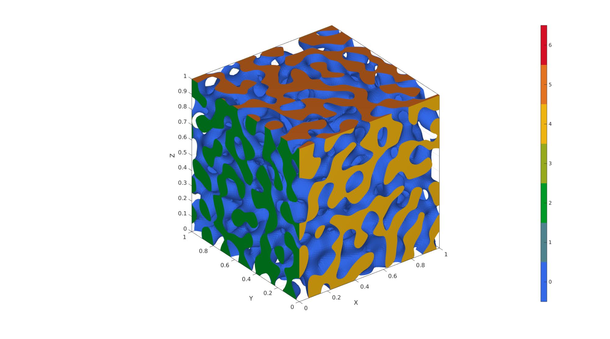
Example 1: Isotropic spinodoid

inputStruct.isocap=true; % option to cap the isosurface
inputStruct.domainSize=1; % domain size
inputStruct.resolution=75; % resolution for sampling GRF
inputStruct.waveNumber=15*pi; % GRF wave number
inputStruct.numWaves=1000; % number of waves in GRF
inputStruct.relativeDensity=0.5; % relative density: between [0.3,1]
inputStruct.thetas=[90 0 0]; % conical half angles (in degrees) along xyz
inputStruct.R = eye(3); % Rotate the GRF, R must be SO(3)

% Create spinodoid
[F,V,C]=spinodoid(inputStruct);

% Using grouping to keep only largest group
groupOptStruct.outputType='label';
[G,~,groupSize]=tesgroup(F,groupOptStruct); %Group connected faces
[~,indKeep]=max(groupSize); %Index of largest group

%Keep only largest group
F=F(G==indKeep,:); %Trim faces
C=C(G==indKeep,:); %Trim color data
[F,V]=patchCleanUnused(F,V); %Remove unused nodes

% Visualize surface
cFigure;
gpatch(F,V,C,'none');
axisGeom; camlight headlight;
colormap gjet; icolorbar;
gdrawnow;

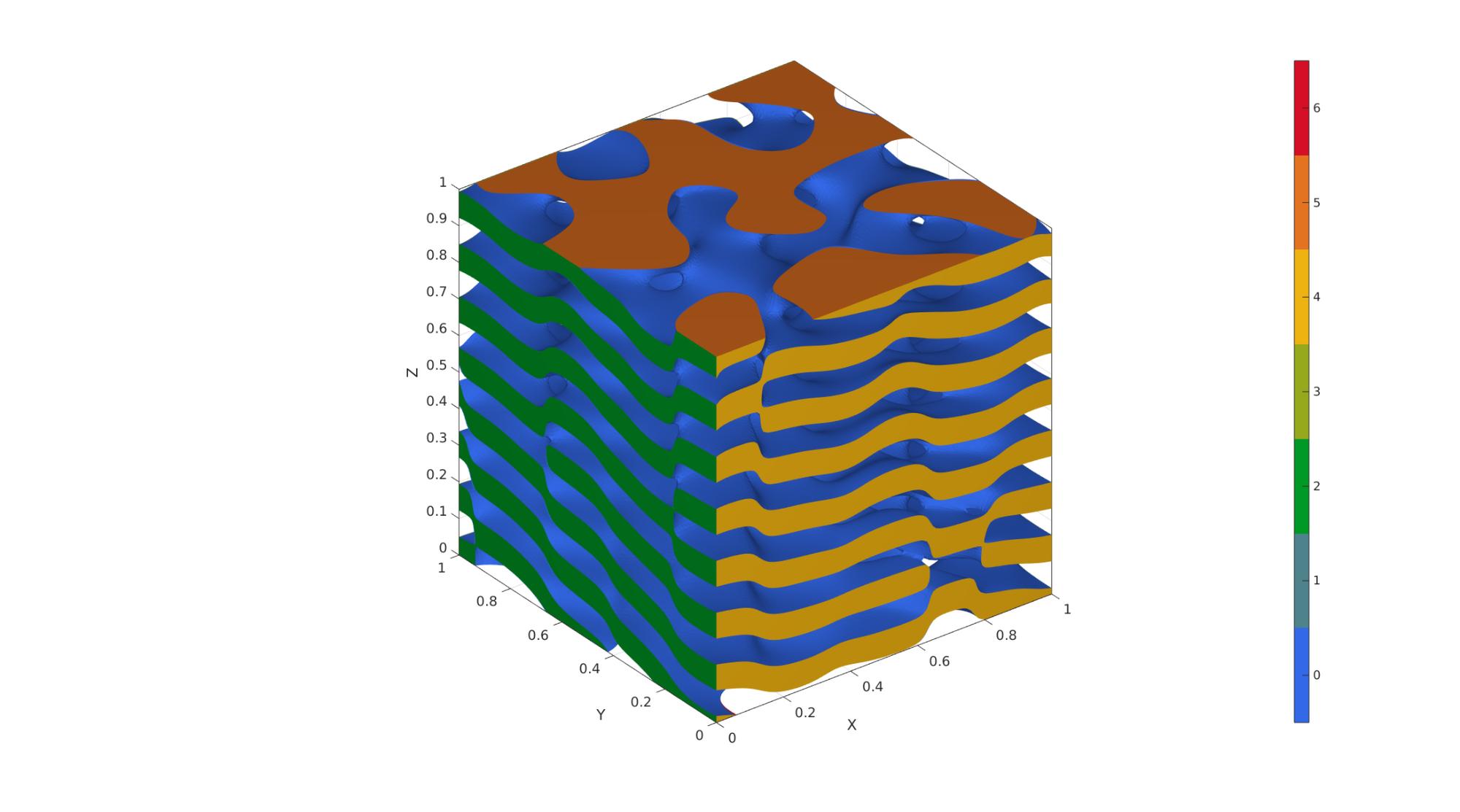
Example 2: Lamellar spinodoid

clear inputStruct; %Clear previous
inputStruct.isocap=true; % option to cap the isosurface
inputStruct.domainSize=1; % domain size
inputStruct.resolution=100; % resolution for sampling GRF
inputStruct.waveNumber=15*pi; % GRF wave number
inputStruct.numWaves=1000; % number of waves in GRF
inputStruct.relativeDensity=0.5; % relative density: between [0.3,1]
inputStruct.thetas=[0 0 30]; % conical half angles (in degrees) along xyz
inputStruct.R = [cos(pi/6),sin(pi/6),0; -sin(pi/6),cos(pi/6),0; 0,0,1]; % Rotate the GRF, R must be SO(3)

% Create spinodoid
[F,V,C]=spinodoid(inputStruct);

% Using grouping to keep only largest group
groupOptStruct.outputType='label';
[G,~,groupSize]=tesgroup(F,groupOptStruct); %Group connected faces
[~,indKeep]=max(groupSize); %Index of largest group

%Keep only largest group
F=F(G==indKeep,:); %Trim faces
C=C(G==indKeep,:); %Trim color data
[F,V]=patchCleanUnused(F,V); %Remove unused nodes

% Visualize surface
cFigure;
gpatch(F,V,C,'none');
axisGeom; camlight headlight;
colormap gjet; icolorbar;
gdrawnow;

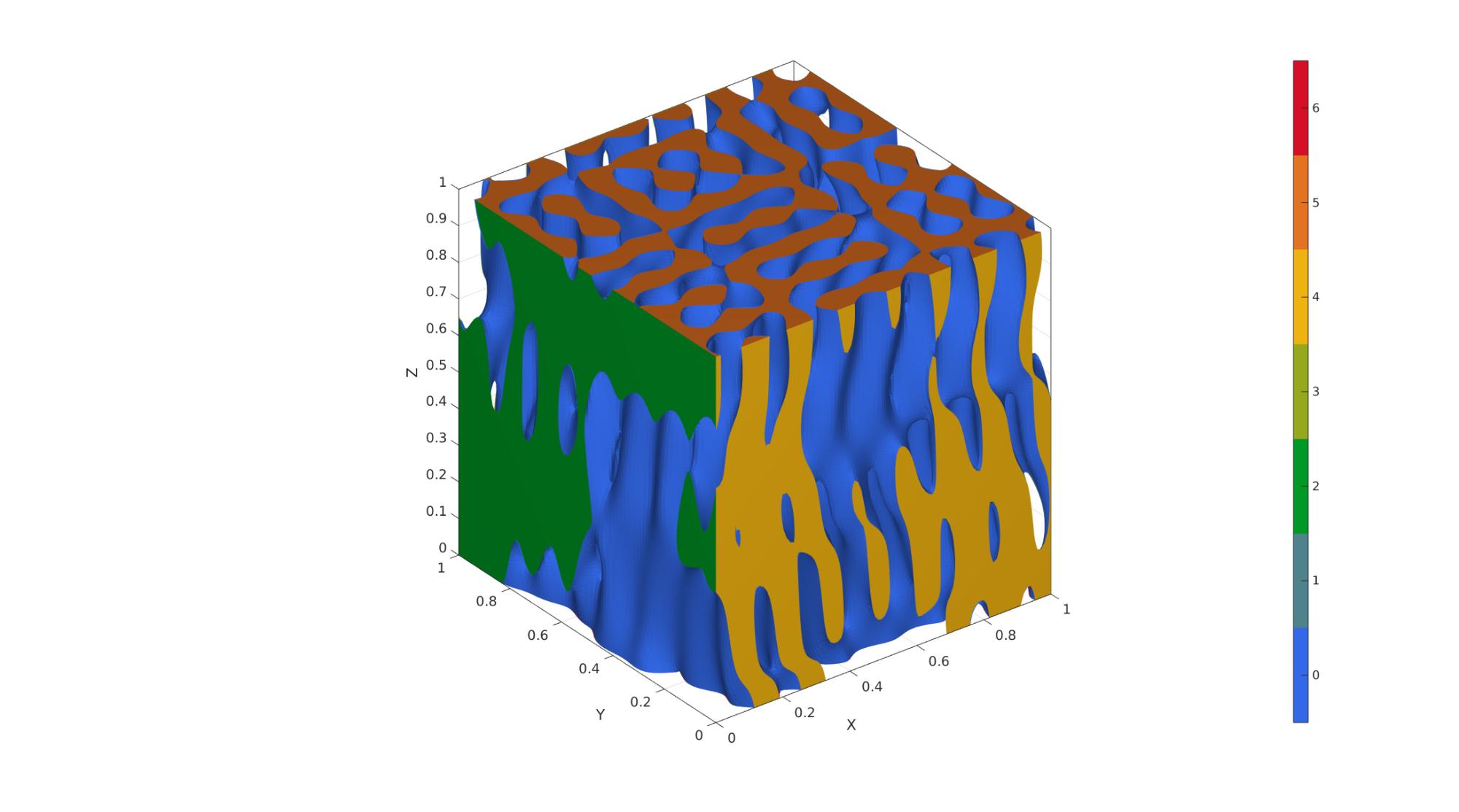
Example 3: Columnar spinodoid

clear inputStruct; %Clear previous
inputStruct.isocap=true; % option to cap the isosurface
inputStruct.domainSize=1; % domain size
inputStruct.resolution=100; % resolution for sampling GRF
inputStruct.waveNumber=15*pi; % GRF wave number
inputStruct.numWaves=1000; % number of waves in GRF
inputStruct.relativeDensity=0.5; % relative density: between [0.3,1]
inputStruct.thetas=[20 15 0]; % conical half angles (in degrees) along xyz
inputStruct.R = eye(3); % Rotate the GRF, R must be SO(3)

% Create spinodoid
[F,V,C]=spinodoid(inputStruct);

% Using grouping to keep only largest group
groupOptStruct.outputType='label';
[G,~,groupSize]=tesgroup(F,groupOptStruct); %Group connected faces
[~,indKeep]=max(groupSize); %Index of largest group

%Keep only largest group
F=F(G==indKeep,:); %Trim faces
C=C(G==indKeep,:); %Trim color data
[F,V]=patchCleanUnused(F,V); %Remove unused nodes

% Visualize surface
cFigure;
gpatch(F,V,C,'none');
axisGeom; camlight headlight;
colormap gjet; icolorbar;
gdrawnow;

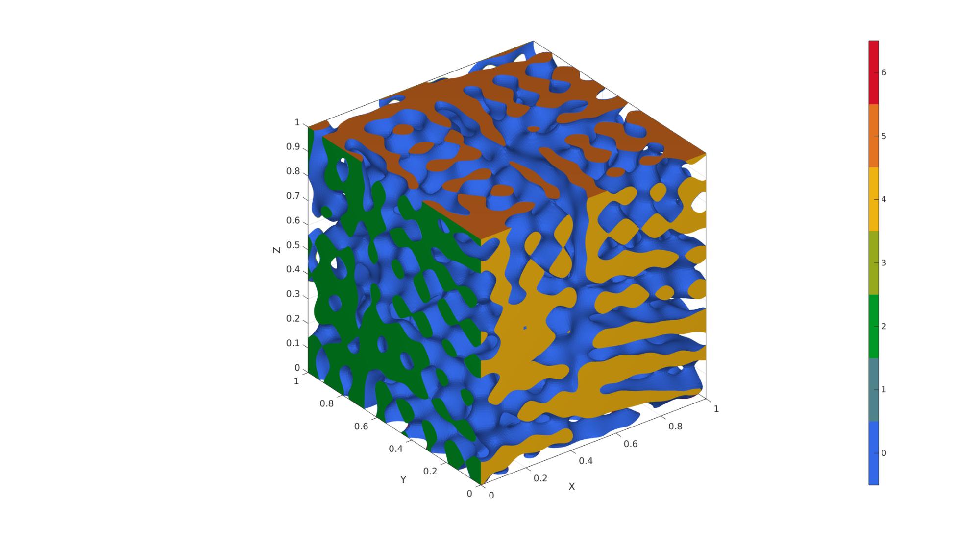
Example 4: Cubic spinodoid

clear inputStruct; %Clear previous
inputStruct.isocap=true; % option to cap the isosurface
inputStruct.domainSize=1; % domain size
inputStruct.resolution=100; % resolution for sampling GRF
inputStruct.waveNumber=15*pi; % GRF wave number
inputStruct.numWaves=1000; % number of waves in GRF
inputStruct.relativeDensity=0.5; % relative density: between [0.3,1]
inputStruct.thetas=[20 20 20]; % conical half angles (in degrees) along xyz
inputStruct.R = eye(3); % Rotate the GRF, R must be SO(3)

% Create spinodoid
[F,V,C]=spinodoid(inputStruct);

% Using grouping to keep only largest group
groupOptStruct.outputType='label';
[G,~,groupSize]=tesgroup(F,groupOptStruct); %Group connected faces
[~,indKeep]=max(groupSize); %Index of largest group

%Keep only largest group
F=F(G==indKeep,:); %Trim faces
C=C(G==indKeep,:); %Trim color data
[F,V]=patchCleanUnused(F,V); %Remove unused nodes

% Visualize surface
cFigure;
gpatch(F,V,C,'none');
axisGeom; camlight headlight;
colormap gjet; icolorbar;
gdrawnow;

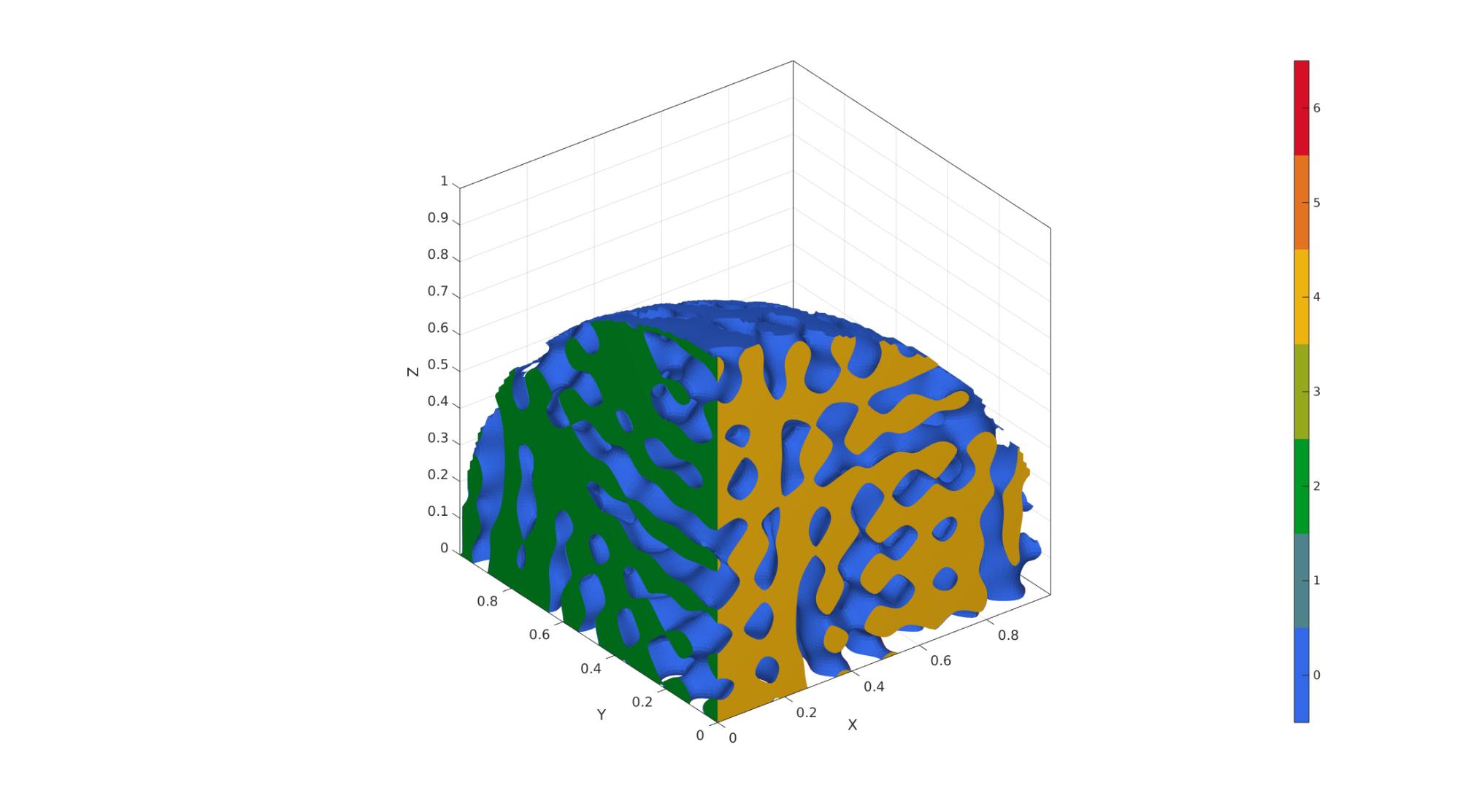
Example 5: Non-cubic domains by specifying "trimDomainFunction"

% In this example, we create a spinodoid in the shape of 1/8th of a sphere
% with radius=1 and centered at (0,0,0). % For this purpose, we first
% create a function with handle trimDomainFunction (preceeded by @) that
% takes as input coordinates (x,y,z) and outputs true if the point lies
% inside the domain and false if outside. Note: x,y,z can be matrices and
% so all operations should be element-wise (denoted by '.').
trimDomainFunction = @(x,y,z)(x.^2+y.^2+z.^2 <= 1^2);

clear inputStruct; %Clear previous
inputStruct.isocap=true; % option to cap the isosurface
inputStruct.domainSize=1; % domain size
inputStruct.resolution=100; % resolution for sampling GRF
inputStruct.waveNumber=15*pi; % GRF wave number
inputStruct.numWaves=1000; % number of waves in GRF
inputStruct.relativeDensity=0.5; % relative density: between [0.3,1]
inputStruct.thetas=[20 20 20]; % conical half angles (in degrees) along xyz
inputStruct.R = eye(3); % Rotate the GRF, R must be SO(3)
inputStruct.trimDomainFunction = trimDomainFunction; % trimDomainFunction

% Create spinodoid
[F,V,C]=spinodoid(inputStruct);

% Using grouping to keep only largest group
groupOptStruct.outputType='label';
[G,~,groupSize]=tesgroup(F,groupOptStruct); %Group connected faces
[~,indKeep]=max(groupSize); %Index of largest group

%Keep only largest group
F=F(G==indKeep,:); %Trim faces
C=C(G==indKeep,:); %Trim color data
[F,V]=patchCleanUnused(F,V); %Remove unused nodes

% Visualize surface
cFigure;
gpatch(F,V,C,'none');
axisGeom; camlight headlight;
colormap gjet; icolorbar;
gdrawnow;

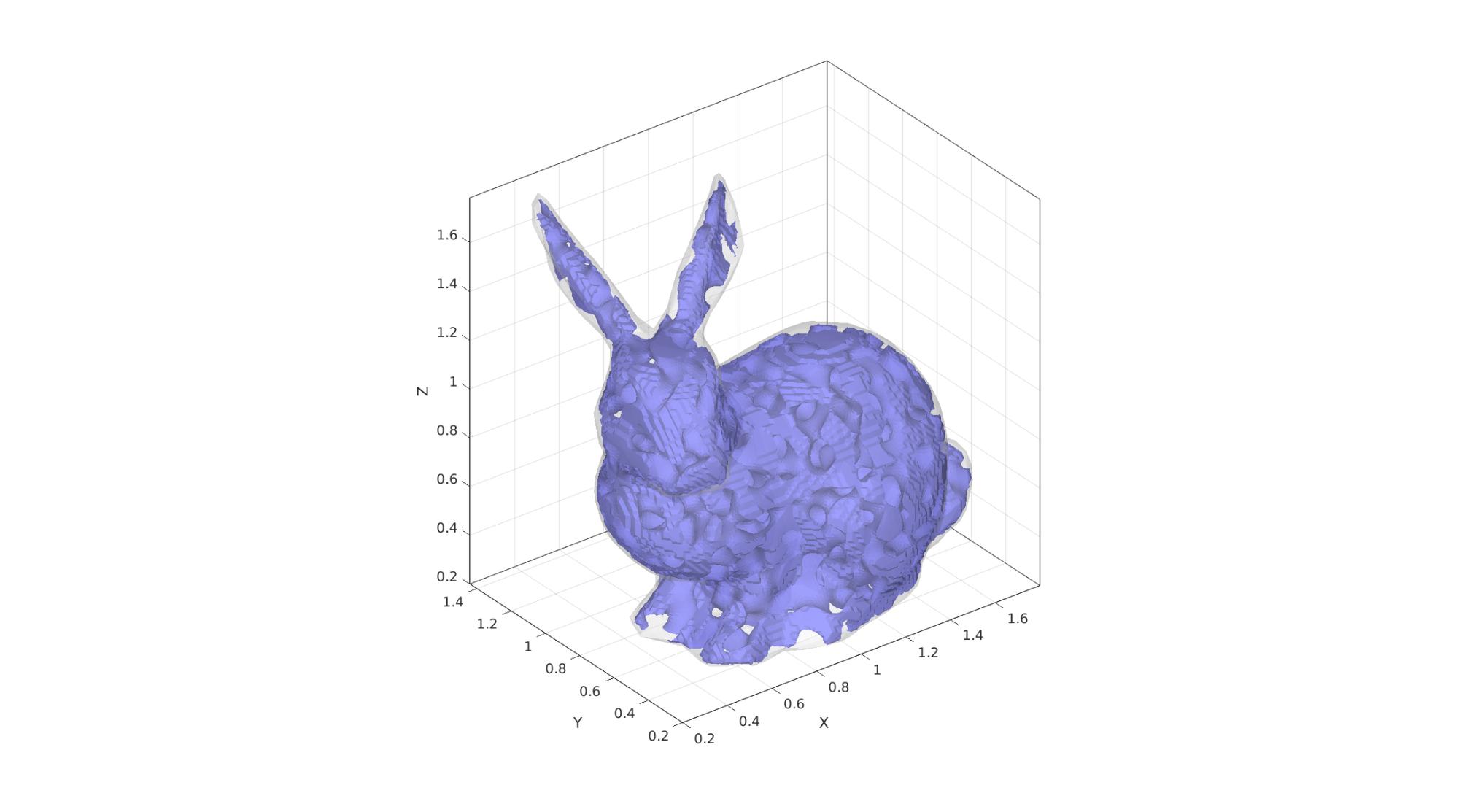
Example 6: Non-cubic domains by specifying a domain surface

domainSize=2;

%Create example domain cropping surface
[Fd,Vd]=stanford_bunny;
Vd=Vd-min(Vd,[],1); %Start at 0
Vd=Vd./max(Vd(:),[],1); %End at 1
Vd=0.1*domainSize+(Vd.*0.8.*domainSize); %Scale to fit in domain

clear inputStruct
inputStruct.isocap=true; % option to cap the isosurface
inputStruct.domainSize=domainSize; % domain size
inputStruct.resolution=150; % resolution for sampling GRF
inputStruct.waveNumber=15*pi; % GRF wave number
inputStruct.numWaves=1000; % number of waves in GRF
inputStruct.relativeDensity=0.5; % relative density: between [0.3,1]
inputStruct.thetas=[90 0 0]; % conical half angles (in degrees) along xyz
inputStruct.R = eye(3); % Rotate the GRF, R must be SO(3)
inputStruct.patchDomain.F=Fd;
inputStruct.patchDomain.V=Vd;

% Create spinodoid
[F,V,C,GRF]=spinodoid(inputStruct);

% Using grouping to keep only largest group
groupOptStruct.outputType='label';
[G,~,groupSize]=tesgroup(F,groupOptStruct); %Group connected faces
[~,indKeep]=max(groupSize); %Index of largest group

%Keep only largest group
F=F(G==indKeep,:); %Trim faces
C=C(G==indKeep,:); %Trim color data
[F,V]=patchCleanUnused(F,V); %Remove unused nodes

% Visualize surface
cFigure;
gpatch(F,V,'bw','none');
gpatch(Fd,Vd,'w','none',0.25);
axisGeom; camlight headlight;
gdrawnow;

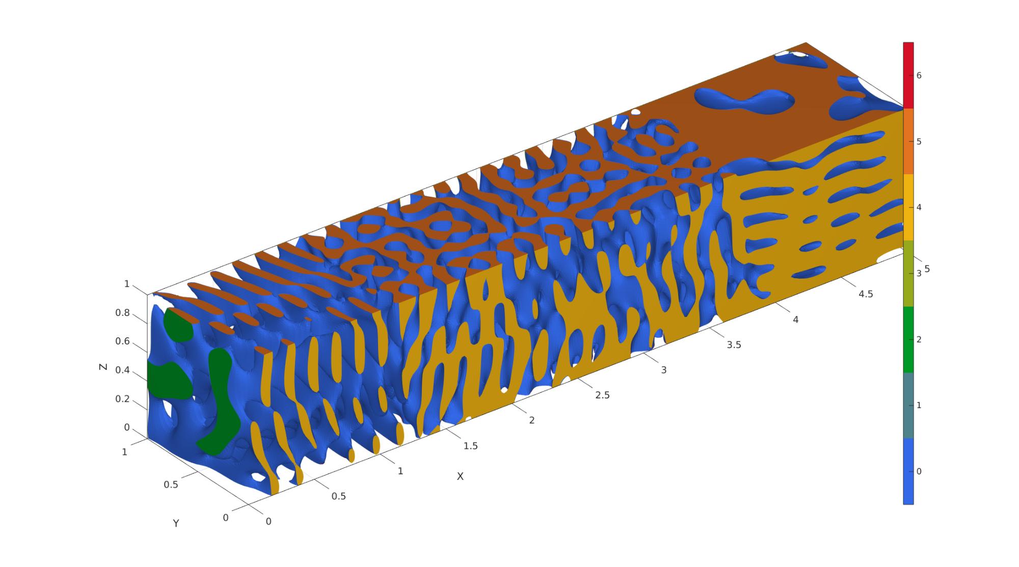
Example 7: Spatially-graded spinodoids

% -----------------------------------------------------------------------
% For reference, see Appendix A of the following paper:
%  L. Zheng, S. Kumar, D.M. Kochmann.
%  Data-driven topology optimization of spinodoid metamaterials with
%  seamlessly tunable anisotropy.
%  Computer Methods in Applied Mechanics and Engineering, 383 (2021), 113894.
%  https://doi.org/10.1016/j.cma.2021.113894
% -----------------------------------------------------------------------

% Example: how to grade 3 spinodoids: A, B, and C

% Set common parameters for 3 different spinodoids
input_A.isocap=true; % option to cap the isosurface
input_A.domainSize=[5,1,1]; % domain size
input_A.resolution=60*input_A.domainSize; % resolution for sampling GRF
input_A.waveNumber=12*pi; % GRF wave number
input_A.numWaves=500; % number of waves in GRF
input_B = input_A;
input_C = input_B;

% Set parameters for individual spinodoids
input_A.relativeDensity=0.3; % relative density: between [0.3,1]
input_A.thetas=[30 0 0]; % conical half angles (in degrees) along

input_B.relativeDensity = 0.5;
input_B.thetas=[30 30 0];

input_C.relativeDensity = 0.8;
input_C.thetas=[0 0 30];

% Compute individual spinodoids
% No need to store faces and vertices, only require underlying GRF,
% grid coordinates, and levelset values
[~,~,~,GRF_A,X,Y,Z,levelset_A]=spinodoid(input_A);
[~,~,~,GRF_B,~,~,~,levelset_B]=spinodoid(input_B);
[~,~,~,GRF_C,~,~,~,levelset_C]=spinodoid(input_C);

% Define the central location of each individual spinodoid in space
% E.g., At center_A, the spinodoid will definitely correspond to input_A.
% As we move away from center_A, it will slowly transition into other
% spinodoids with input_B and input_C.
center_A = [0.0, 0.5, 0.0];
center_B = [2.5, 0.5, 0.5];
center_C = [5.0, 0.5, 1.0];

% kappa controls the lengthscale of transition between spinodoids
% Higher kappa => faster transition
% Lower kappa => slower transition
kappa = 10;

% Using Gaussian (a.k.a. radial basis functions) interpolation.
% One can use any interpolation scheme of choice as long as weights at
% every grid point sum up to 1.
% Computing the weights for each spinodoid evaluated on all grid points.
weights_A = exp(-kappa * squared_distance_from_point(X,Y,Z,center_A));
weights_B = exp(-kappa * squared_distance_from_point(X,Y,Z,center_B));
weights_C = exp(-kappa * squared_distance_from_point(X,Y,Z,center_C));
% Weights must sum up to 1.
sum_weights = weights_A + weights_B + weights_C;
weights_A = weights_A ./ sum_weights;
weights_B = weights_B ./ sum_weights;
weights_C = weights_C ./ sum_weights;

% Interpolating using the above weights
graded_GRF =  weights_A .* (GRF_A - levelset_A) ...
            + weights_B .* (GRF_B - levelset_B) ...
            + weights_C .* (GRF_C - levelset_C);

% Compue isosurface
graded_levelset = 0;
[f,v] = isosurface(X,Y,Z,graded_GRF,graded_levelset);
c=zeros(size(f,1),1);

% Compute isocaps
[fc,vc] = isocaps(X,Y,Z,graded_GRF,graded_levelset,'enclose','below');

% Boilerplate code for preparing output for exporting/visualization
nc=patchNormal(fc,vc);
cc=zeros(size(fc,1),1);
cc(nc(:,1)<-0.5)=1;
cc(nc(:,1)>0.5)=2;
cc(nc(:,2)<-0.5)=3;
cc(nc(:,2)>0.5)=4;
cc(nc(:,3)<-0.5)=5;
cc(nc(:,3)>0.5)=6;

% Join sets
[f,v,c]=joinElementSets({f,fc},{v,vc},{c,cc});

% Merge nodes
[f,v]=mergeVertices(f,v);

% Check for unique faces
[~,indUni,~]=unique(sort(f,2),'rows');
f=f(indUni,:); %Keep unique faces
c=c(indUni);

% Remove collapsed faces
[f,logicKeep]=patchRemoveCollapsed(f);
c=c(logicKeep);

% Remove unused points
[f,v]=patchCleanUnused(f,v);

% Invert faces
f=fliplr(f);

%Visualize
vizualize_graded_spinodoid(f,v,c)

% Compute squared distance from a point
function [sq_dist] = squared_distance_from_point(X,Y,Z,point)
% X, Y, Z are 3D matrices
% point is a 1x3 vector
sq_dist = (X-point(1)).^2 + (Y-point(2)).^2 + (Z-point(3)).^2;
end

function [] = vizualize_graded_spinodoid(F,V,C)

% Using grouping to keep only largest group
groupOptStruct.outputType='label';
[G,~,groupSize]=tesgroup(F,groupOptStruct); %Group connected faces
[~,indKeep]=max(groupSize); %Index of largest group

%Keep only largest group
F=F(G==indKeep,:); %Trim faces
C=C(G==indKeep,:); %Trim color data
[F,V]=patchCleanUnused(F,V); %Remove unused nodes

% Visualize surface
cFigure;
gpatch(F,V,C,'none');
axisGeom; camlight headlight;
colormap gjet; icolorbar;
gdrawnow;

end

GIBBON www.gibboncode.org

Kevin Mattheus Moerman, [email protected]

GIBBON footer text

License: https://github.com/gibbonCode/GIBBON/blob/master/LICENSE

GIBBON: The Geometry and Image-based Bioengineering add-On. A toolbox for image segmentation, image-based modeling, meshing, and finite element analysis.

Copyright (C) 2006-2023 Kevin Mattheus Moerman and the GIBBON contributors

This program is free software: you can redistribute it and/or modify it under the terms of the GNU General Public License as published by the Free Software Foundation, either version 3 of the License, or (at your option) any later version.

This program is distributed in the hope that it will be useful, but WITHOUT ANY WARRANTY; without even the implied warranty of MERCHANTABILITY or FITNESS FOR A PARTICULAR PURPOSE. See the GNU General Public License for more details.

You should have received a copy of the GNU General Public License along with this program. If not, see http://www.gnu.org/licenses/.

Published with MATLAB® R2023a