im2cart

Below is a demonstration of the features of the im2cart function

Syntax
Description
Examples
Example: 2D image coordinate systems
Example: 3D image coordinate handling and visualization

clear; close all; clc;

Syntax

[X,Y,Z]=im2cart(I,J,K,v);

[X,Y,Z]=im2cart(I,J,K);

[V_xyz]=im2cart(V_ijk,v);

[V_xyz]=im2cart(V_ijk);

[V_xyz]=im2cart(V_ij);

Description

This function converts the image coordinates I,J,K to the cartesian coordinates X,Y,Z using the voxel dimension v.

I,J,K can be scalars, vectors or matrices. v is a vector of length 3 where v(1), v(2) and v(3) correspond to the voxel dimensions in the x,y and z direction respectively.

This function maps the row, column, slice coordinates I,J,K to "real-world" Cartesian coordinates X,Y,Z based on: X=(J-0.5).*v(2); Y=(I-0.5).*v(1); Z=(K-0.5).*v(3);

Note that the columns relate to X while rows relate to Y.

A single coordinate array may also be specified whereby the columns define the I, J, and K coordinates. If a single output is requested the output will also consist of such an array whereby columns are the X, Y, and Z coordinates

Examples

Plot settings

cMap=gjet(250);
faceAlpha1=1;
faceAlpha2=0.65;
fontSize=25;

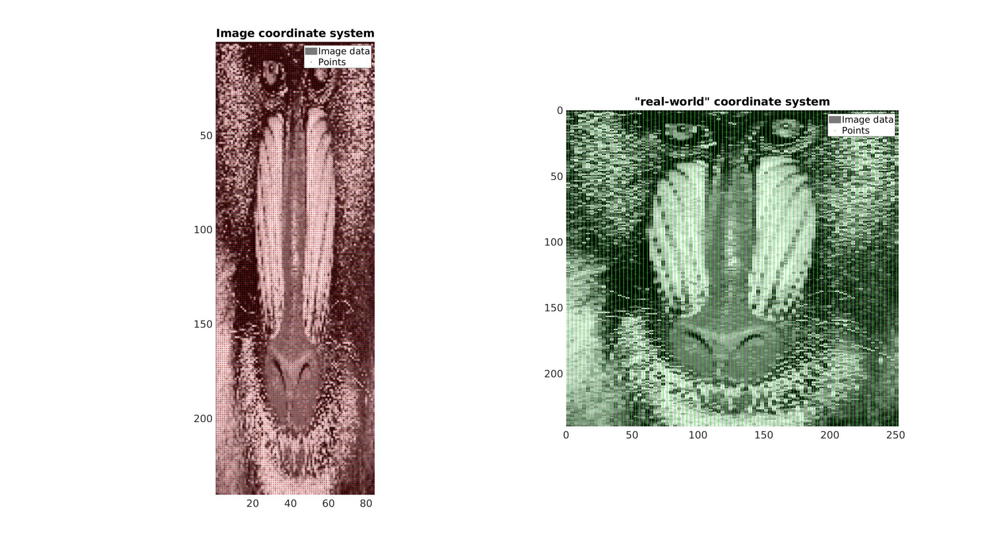
Example: 2D image coordinate systems

In this example a 2D image with an anisotropic voxel (pixel) size is used. It is first visualized in image coordinates which, since voxel size is not taken in to account , appears stretcged. Next it is also visualized using "real-world" Cartesian coordinates which do take the real anisotropic voxel size into account (using im2cart). This image appears unstretched.

Get example image data

imageData=load('mandrill'); %Image data for photograph
M=double(imageData.X); %Get gray scale intensity information
M=M(1:2:end,1:6:end); %Reduce density of image and make anisotropic
v=[1 3 1]; %example voxel size

Create row (I) and column (J) image coordinates for all voxel centers

[I,J]=ndgrid(1:1:size(M,1),1:1:size(M,2)); %Row and column coordinates
K=ones(size(I)); %Slice coordinates
P_IJ=[I(:) J(:) K(:)]; %The collected coordinate array

Use im2cart to convert to "Cartesian" or real world coordinates

P_XY=im2cart(P_IJ,v); %Real world coordinates.

Create patch data for plotting

%Get patch data
[F,V,C]=im2patch(M,true(size(M)),'sk');

Use im2cart to convert to "Cartesian" or real world coordinates

V_XY=im2cart(V(:,[2 1 3]),v);

Visualize

cFigure;
subplot(1,2,1); hold on;
title('Image coordinate system');
hp1=gpatch(F,V,C,'none');
hp2=plotV(P_IJ(:,[2 1 3]),'r.','markerSize',5);
legend([hp1,hp2],{'Image data','Points'})
axis ij; axis tight; axis equal;
set(gca,'FontSize',fontSize);
colormap gray;

subplot(1,2,2); hold on;
title('"real-world" coordinate system');
hp1=gpatch(F,V_XY,C,'none');
hp2=plotV(P_XY,'g.','markerSize',5);
legend([hp1,hp2],{'Image data','Points'})
axis ij; axis tight; axis equal;
set(gca,'FontSize',fontSize);
colormap gray;

drawnow;

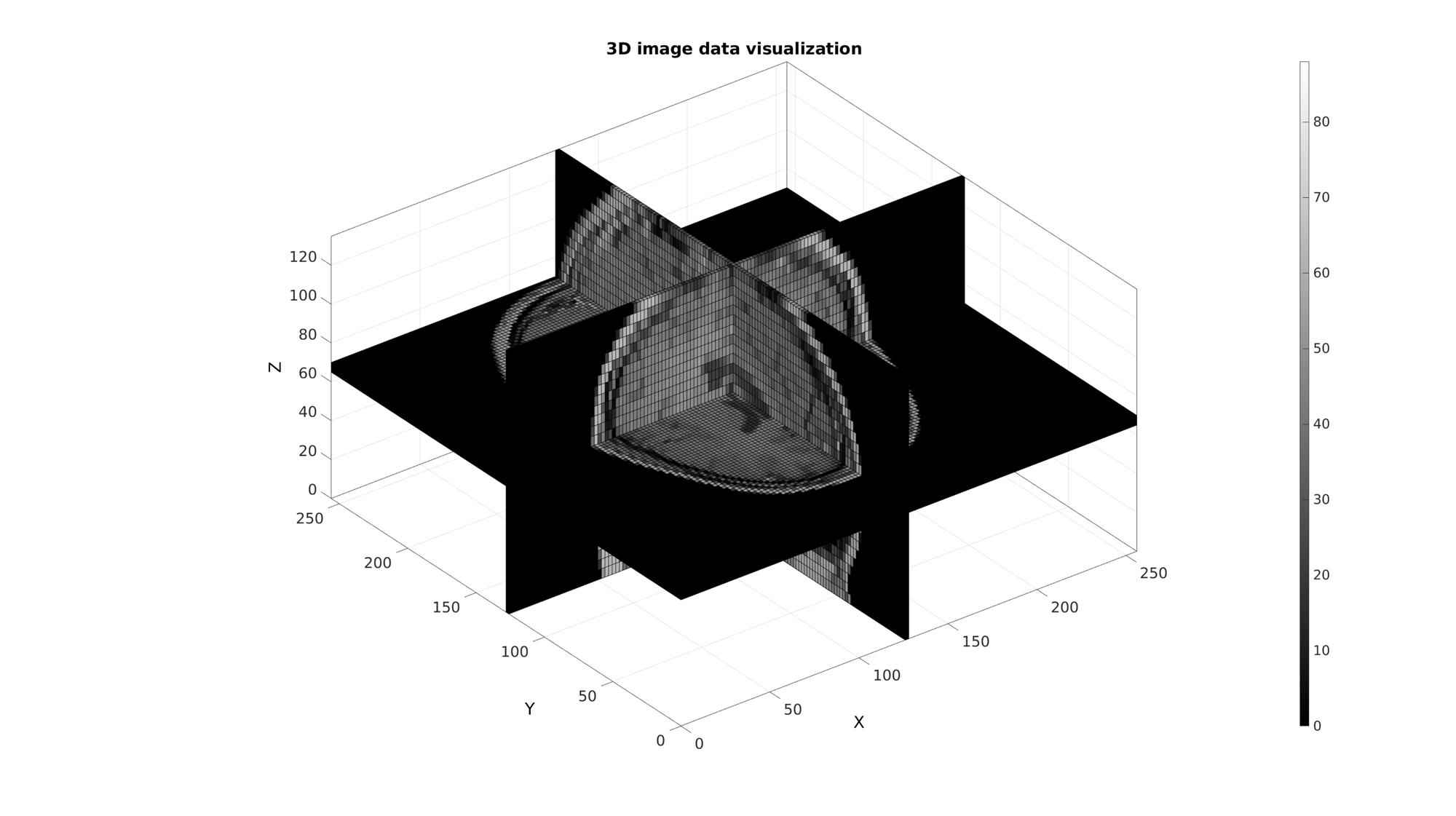
Example: 3D image coordinate handling and visualization

Get example image data

load mri;
M=squeeze(D); %example image data set
v=[2 2 5]; %example voxel size, note voxels are ellongated in slice direction

Use im2patch to get coordinates of voxel data for plotting

%Defining row, column and slice indicices for slice patching
sliceIndexI=round(size(M,1)/2); %(close to) middle row
sliceIndexJ=round(size(M,2)/2); %(close to) middle column
sliceIndexK=round(size(M,3)/2); %(close to) middle slice

logicPlot=false(size(M));
logicPlot(sliceIndexI,:,:)=1;
logicPlot(:,sliceIndexJ,:)=1;
logicPlot(:,:,sliceIndexK)=1;

%Get patch data
[F,V,C]=ind2patch(logicPlot,M,'vb');

Use im2cart to scale coordinates based on voxel size. The patch data consists of a matrix array defining the faces, a matrix array defining the vertices and a vector for the colour data. The vertices are based on the image coordinates however they are formatted as: [X(:) Y(:) Z(:)]. X relates to columns, Y to rows and Z to slices.

% Convert image coordinates to cartesian coordinates
[V(:,1),V(:,2),V(:,3)]=im2cart(V(:,2),V(:,1),V(:,3),v);

Visualize

cFigure;
title('3D image data visualization');
xlabel('X (mm)');ylabel('Y (mm)'); zlabel('Z (mm)'); hold on;
gpatch(F,V,C);
axisGeom(gca,fontSize);
colormap(gray(250)); colorbar;
camlight headlight;
drawnow;

GIBBON www.gibboncode.org

Kevin Mattheus Moerman, [email protected]

GIBBON footer text

License: https://github.com/gibbonCode/GIBBON/blob/master/LICENSE

GIBBON: The Geometry and Image-based Bioengineering add-On. A toolbox for image segmentation, image-based modeling, meshing, and finite element analysis.

This program is free software: you can redistribute it and/or modify it under the terms of the GNU General Public License as published by the Free Software Foundation, either version 3 of the License, or (at your option) any later version.

This program is distributed in the hope that it will be useful, but WITHOUT ANY WARRANTY; without even the implied warranty of MERCHANTABILITY or FITNESS FOR A PARTICULAR PURPOSE. See the GNU General Public License for more details.