DEMO_volumetric_SED_eval

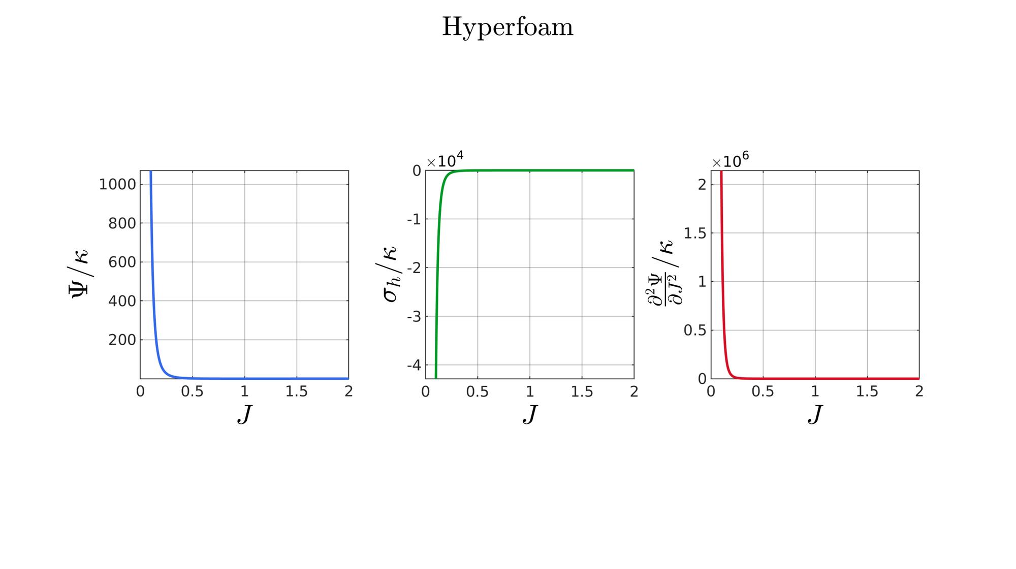
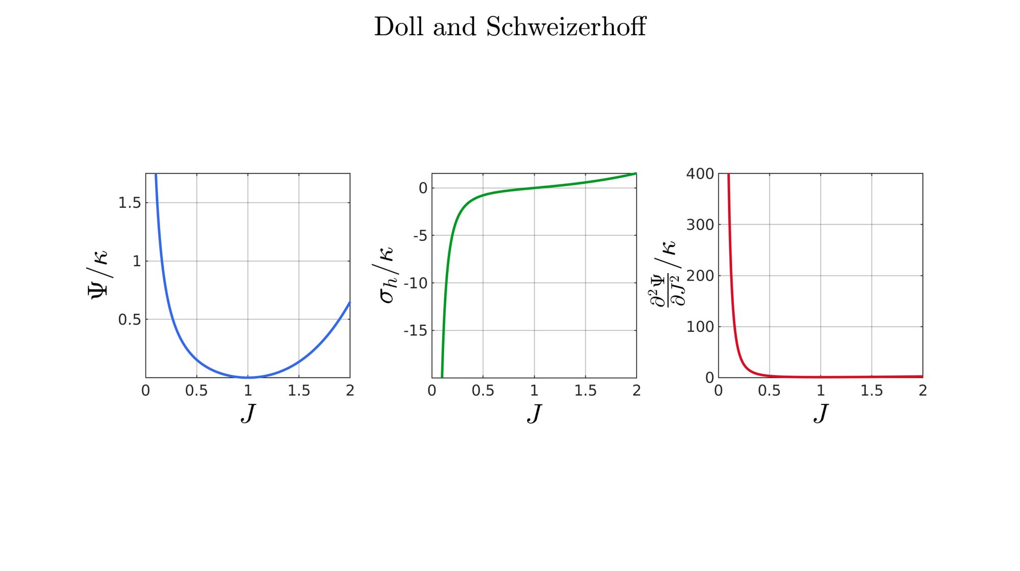
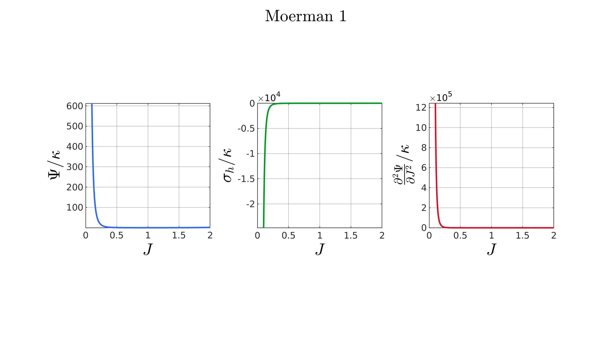
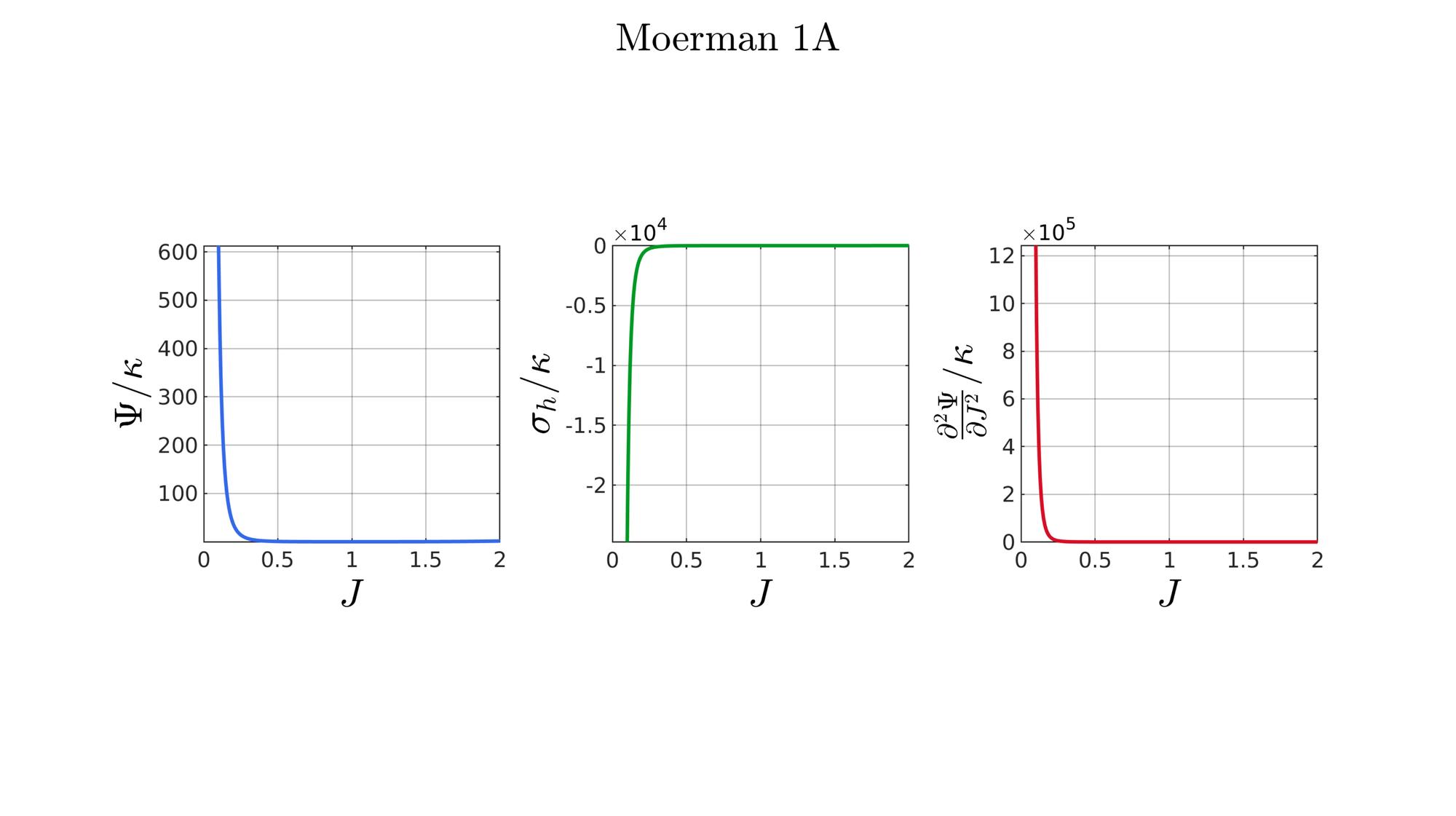
This demo was developed as part of the paper: Moerman et al. "Novel Hyperelastic Models for Large Volumetric Deformations".

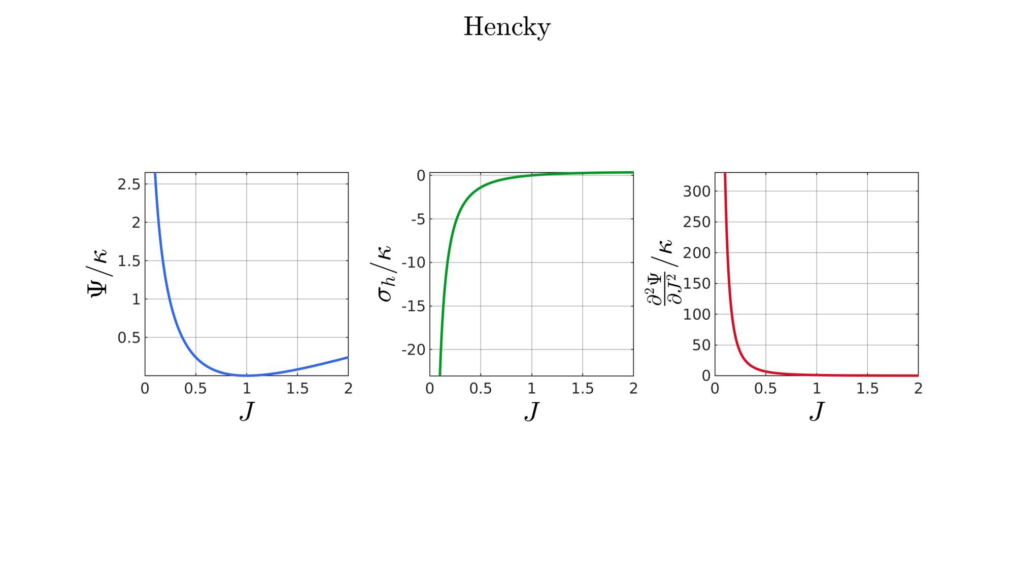
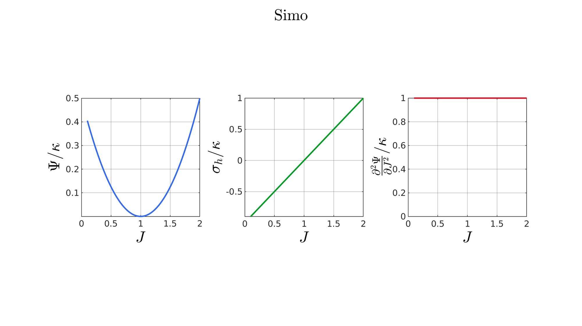
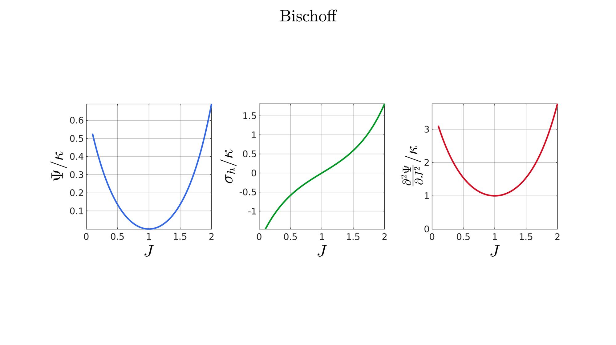
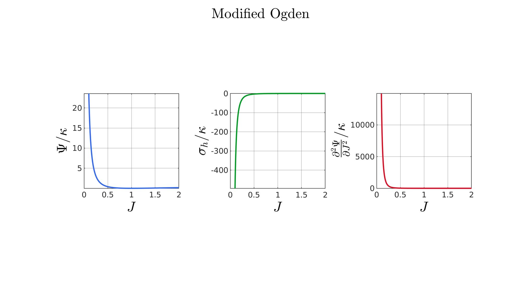
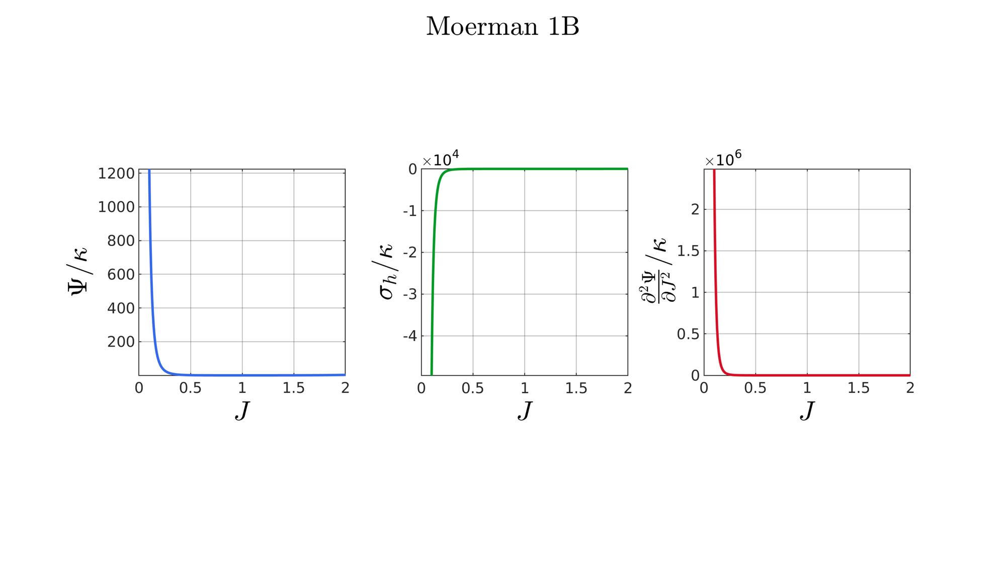
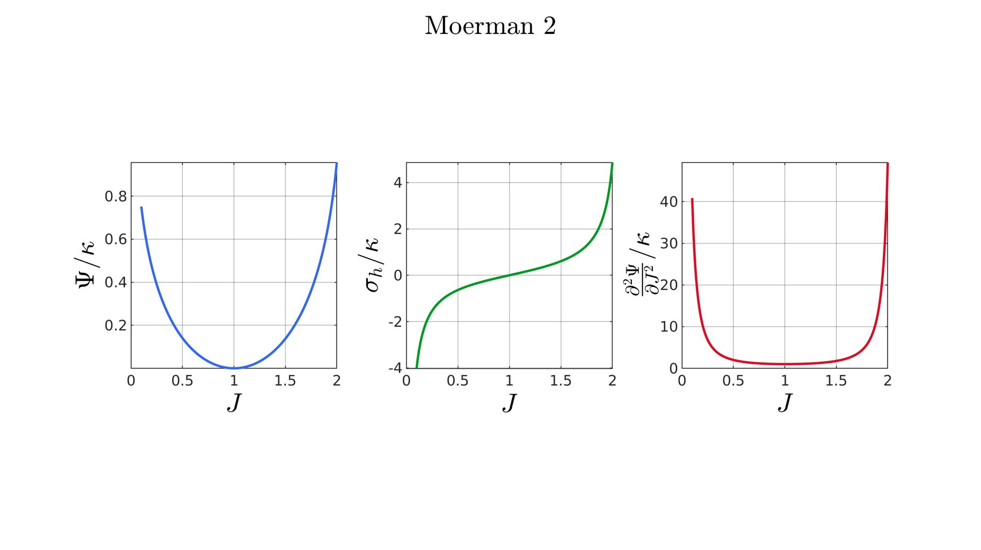
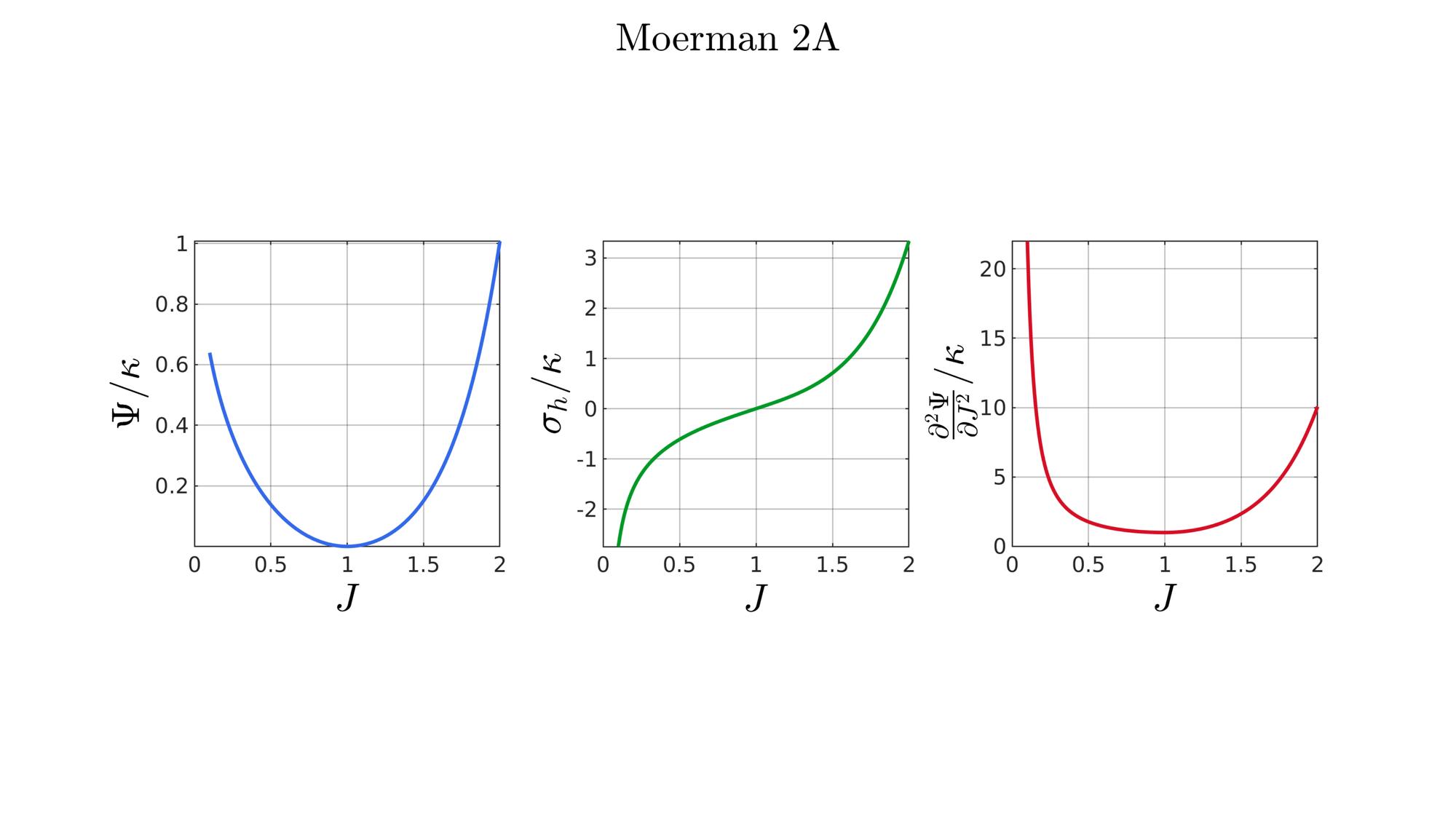
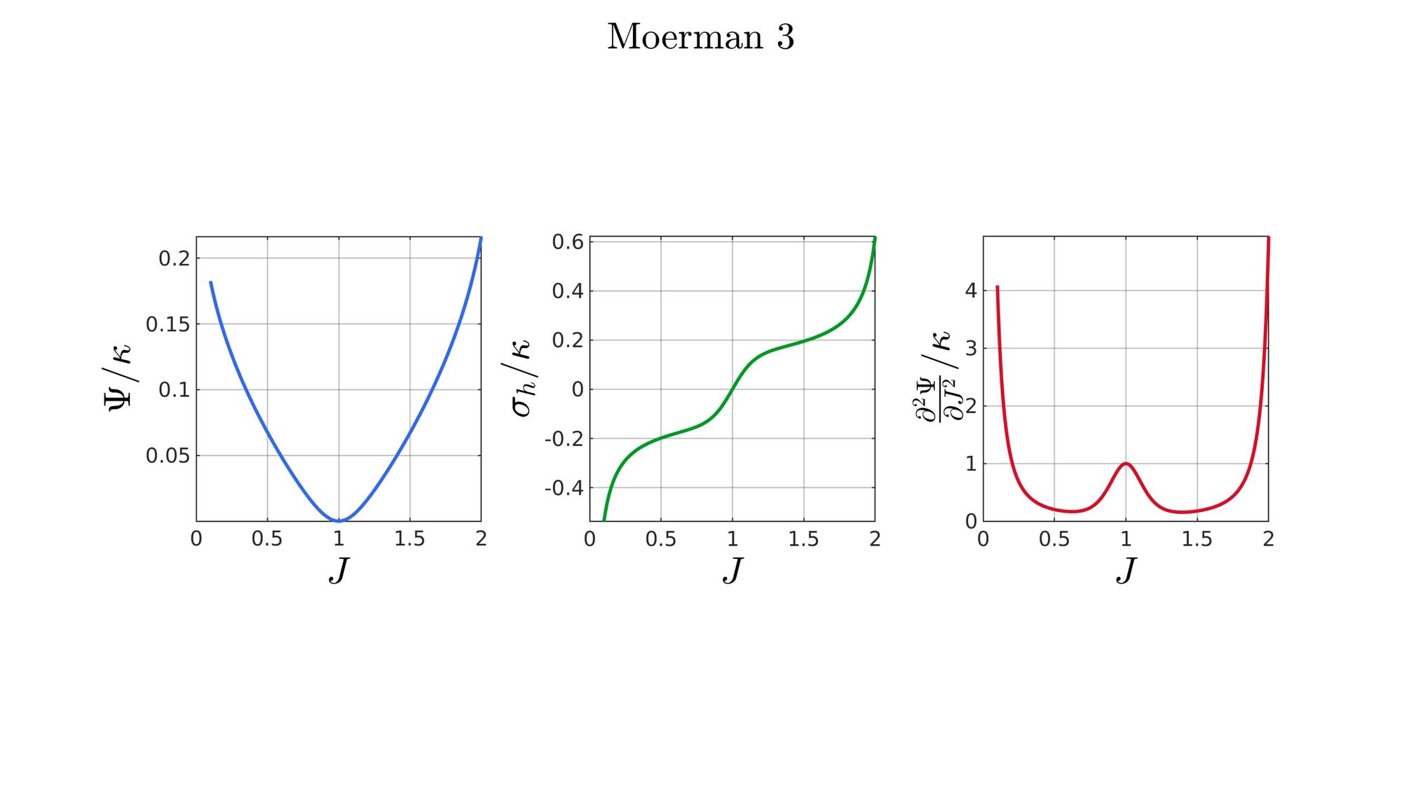
The demo features: * Implementations of hyperelastic volumetric strain energy density functions (SEDs) * Visualizations of the SED, hydrostatic stress, and tangent as a function of the volume ratio.

Contents

Keywords

clear; close all; clc;

Plot settings

fontSize=36;
fontSizeInner=fontSize+15;
fontSizeLabel=fontSize+30;
plotColors=gjet(4);
plotColors=plotColors([1 2 4],:);

lineWidth=6;
gridAlpha=0.3;
LineWidthAxis=2;
legendHeight=0.05;
numXTicks=5;

Control parameters

formulationCases=1:12;  %Choose formulation 1:12
k=1; %Default bulk modulus (except for hyperfoam)

J_max=2;
numPoints=2000; %Number of points for plotting
J=linspace(0.1,J_max,numPoints)'; %The volume ratios
xtickRange=linspace(0,max(J),numXTicks); %X-axis tick range

Get or set formulation specific data and parameters

for formulationCase=formulationCases

    switch formulationCase
        case 1 %Hencky
            formulationName='Hencky';
            parSet(1)=k; %Bulk modulus
        case 2 %Simo
            formulationName='Simo';
            parSet(1)=k; %Bulk modulus
        case 3 %Bischoff
            formulationName='Bischoff';
            b=2; %Beta
            parSet(1)=k; %Bulk modulus
            parSet(2)=b; %Beta
        case 4 %Modified Ogden
            formulationName='Modified Ogden';
            b=2;%Beta
            parSet(1)=k; %Bulk modulus
            parSet(2)=b; %Beta
        case 5 %Hyperfoam
            formulationName='Hyperfoam';
            mu=1;
            a=2; %Alpha
            b=2; %Beta
            parSet(1)=mu; %Mu
            parSet(2)=a; %Alpha
            parSet(3)=b; %Beta
        case 6 %Doll and Schweizerhoff
            formulationName='Doll and Schweizerhoff';
            a=3; %Alpha
            b=2; %Beta
            parSet(1)=k; %Bulk modulus
            parSet(2)=a; %Alpha
            parSet(3)=b; %Beta
        case 7 %Moerman 1
            formulationName='Moerman 1';
            b1=3;
            b2=2;
            parSet(1)=k; %Bulk modulus
            parSet(2)=b1; %Alpha
            parSet(3)=b2; %Beta
        case 8 %Moerman 1A
            formulationName='Moerman 1A';
            b1=3;
            b2=2;
            q=0.5;
            parSet(1)=k; %Bulk modulus
            parSet(2)=b1; %Alpha
            parSet(3)=b2; %Beta
            parSet(4)=q; %Weigthing factor
        case 9 %Moerman 1B
            formulationName='Moerman 1B';
            b1=3;
            b2=2;
            parSet(1)=k; %Bulk modulus
            parSet(2)=b1; %Alpha
            parSet(3)=b2; %Beta
        case 10 %Moerman 2
            formulationName='Moerman 2';
            J1=max(J)+0.1;
            J2=0;
            parSet(1)=k; %Bulk modulus
            parSet(2)=J1; %J1
            parSet(3)=J2; %J2
        case 11 %Moerman 2A
            formulationName='Moerman 2A';
            b1=3;
            b2=2;
            parSet(1)=k; %Bulk modulus
            parSet(2)=b1; %Alpha
            parSet(3)=b2; %Beta
        case 12 %Moerman 3
            formulationName='Moerman 3';
            J1=max(J)+0.1;
            J2=0;
            s1=0.15;
            s2=0.15;
            q1=0.9;
            q2=0.9;
            parSet(1)=k; %Bulk modulus
            parSet(2)=J1; %J1
            parSet(3)=J2; %J2
            parSet(4)=s1; %s1
            parSet(5)=s2; %s2
            parSet(6)=q2; %q1
            parSet(7)=q2; %q2
    end

Calculate SED

    %Get normalized SED
    [W,S,T]=SED_eval(formulationCase,parSet,J);

Visualize data

    hf=cFigure;
    ht=suptitle(formulationName);
    ht.FontSize=fontSizeLabel;
    ht.Interpreter='latex';

    subplot(1,3,1); hold on;
    set(gca,'FontSize',fontSize,'LineWidth',LineWidthAxis,'GridAlpha',gridAlpha);
    xlabel('$J$','FontSize',fontSizeLabel,'Interpreter','latex');
    ylabel('$\Psi/\kappa$','FontSize',fontSizeLabel,'Interpreter','latex');

    hp1=plot(J,W,'k-','LineWidth',lineWidth);
    hp1.Color=plotColors(1,:);

    grid on; axis tight; axis square; box on;
    xlim([0 max(J(:))]);
    set(gca,'XTick',xtickRange);

    subplot(1,3,2); hold on;
    set(gca,'FontSize',fontSize,'LineWidth',LineWidthAxis,'GridAlpha',gridAlpha);
    xlabel('$J$','FontSize',fontSizeLabel,'Interpreter','Latex');
    ylabel('$\sigma_{h}/\kappa$','FontSize',fontSizeLabel,'Interpreter','Latex');
    grid on; axis tight; axis square; box on;

    hp2=plot(J,S,'k-','LineWidth',lineWidth);
    hp2.Color=plotColors(2,:);

    grid on; axis tight; axis square; box on;
    xlim([0 max(J(:))]);
    set(gca,'XTick',xtickRange);

    subplot(1,3,3); hold on;
    set(gca,'FontSize',fontSize,'LineWidth',LineWidthAxis,'GridAlpha',gridAlpha);
    xlabel('$J$','FontSize',fontSizeLabel,'Interpreter','latex');
    ylabel('$\frac{\partial^2 \Psi}{\partial J^2} /\kappa$','FontSize',fontSizeLabel,'Interpreter','Latex');

    hp3=plot(J,T,'k-','LineWidth',lineWidth);
    hp3.Color=plotColors(3,:);

    grid on; axis tight; axis square; box on;
    xlim([0 max(J(:))]);
    ylim([0 max(T(:))]);
    set(gca,'XTick',xtickRange);

    drawnow;

end

Evaluate SED

function [W,S,T]=SED_eval(formulationCase,parSet,J)

switch formulationCase
    case 1 %Hencky
        k=parSet(1);
        W=k/2*log(J).^2;
        S=k*log(J)./J;
        T=(k-k*log(J))./J.^2;
    case 2 %Simo
        k=parSet(1);
        W=(k/2).*(J-1).^2;
        S=(k/2).*(2*J-2);
        T=k*ones(size(J));
    case 3 %Bischoff
        k=parSet(1);
        b=parSet(2);
        W=(k./b.^2).*(cosh(b*(J-1))-1);
        S=(k./b)   .* sinh(b*(J-1));
        T=k           .* cosh(b*(J-1));
    case 4 %Modified Ogden
        k=parSet(1);
        b=parSet(2);
        W=(k./b.^2).*(J.^-b - 1 + b.*log(J));
        S=(k./b)   .*(1./J     - J.^(-b-1));
        T=(k./b)   .*(-1./J.^2  + (b+1).*J.^(-b-2));
    case 5 %Hyperfoam
        mu=parSet(1);
        a=parSet(2);
        b=parSet(3);
        k=mu.*(b+1/3);
        W=(2*mu./(a.^2)).*( 3*(J.^(a/3)-1)...
            +(1./b.*( (J.^(-a.*b))-1 )) );
        S=(1./J).*(2*mu./a).*(J.^(a/3)...
            -J.^(-a.*b) );
        T=(1./(J.^2)).*(2*mu/a).*((a./3-1).*J.^(a./3) +...
            (a.*b+1).*J.^(-a*b) );
    case 6 %Doll and Schweizerhoff
        k=parSet(1);
        a=parSet(2);
        b=parSet(3);
        W=( (k/(a+b)).*( ((1/(a+1)).*(J.^(a+1))) + ((1/(b-1)).*(J.^(-b+1)))) )...
            -(k.*(1/(a+1)).*(1/(b-1)));
        S=(k/(a+b)).*(J.^a-J.^(-b));
        T=(k/(a+b)).*(a*J.^(a-1)+b*J.^(-b-1));
    case 7 %Moerman 1
        k=parSet(1);
        b1=parSet(2);
        b2=parSet(3);
        W=(k/4)      .*( (1/b1^2).*((J.^ b1)-1).^2 + ...
            (1/b2^2).*((J.^-b2)-1).^2 );
        S=(k/2)./J   .*( (1/b1  ).*(J.^( 2*b1) - J.^b1 ) - ...
            (1/b2  ).*(J.^(-2*b2) - J.^-b2) );
        T=(k/2)./J.^2.*( ((2-1/b1)*J.^( 2*b1)-(1-1/b1)*J.^b1) + ...
            ((2+1/b2)*J.^(-2*b2)-(1+1/b2)*J.^-b2) );
    case 8 %Moerman 1A
        k=parSet(1);
        b1=parSet(2);
        b2=parSet(3);
        q=parSet(4);

        W1=(k/(2*b1^2)).*(  q).*((J.^ b1)-1).^2;
        W2=(k/(2*b2^2)).*(1-q).*((J.^-b2)-1).^2;
        W=W1+W2;

        S1= (k/b1)./J.*(  q).*(J.^( 2*b1)-J.^b1 );
        S2=-(k/b2)./J.*(1-q).*(J.^(-2*b2)-J.^-b2);
        S=S1+S2;

        T1=(k./J.^2).*(  q).*((2-1/b1)*J.^( 2*b1)-(1-1/b1)*J.^b1 );
        T2=(k./J.^2).*(1-q).*((2+1/b2)*J.^(-2*b2)-(1+1/b2)*J.^-b2);
        T=T1+T2;
    case 9 %Moerman 1B
        k=parSet(1);
        b1=parSet(2);
        b2=parSet(3);

        L1=(J>=1);
        L2=(J<1);

        W=zeros(size(J));
        W(L1)=(k/(2*b1^2)).*((J(L1).^ b1)-1).^2;
        W(L2)=(k/(2*b2^2)).*((J(L2).^-b2)-1).^2;

        S=zeros(size(J));
        S(L1)= (k/b1).*(J(L1).^( 2*b1-1)-J(L1).^( b1-1));
        S(L2)=-(k/b2).*(J(L2).^(-2*b2-1)-J(L2).^(-b2-1));

        T=zeros(size(J));
        T(L1)=(k/b1).*((2*b1-1)*J(L1).^( 2*b1-2)-(b1-1)*J(L1).^( b1-2));
        T(L2)=(k/b2).*((2*b2+1)*J(L2).^(-2*b2-2)-(b2+1)*J(L2).^(-b2-2));
    case 10 %Moerman 2
        k=parSet(1);
        J1=parSet(2);
        J2=parSet(3);

        a1=(2/pi)*(J1-1);
        a2=(2/pi)*(J2-1);

        W1=(-k*a1.^2)*log(cos((J-1)/a1));
        W2=(-k*a2.^2)*log(cos((J-1)/a2));

        W=zeros(size(W1));
        W(J>=1)=W1(J>=1);
        W(J<1)=W2(J<1);
        W=real(W);
        W(J>=J1)=inf;
        W(J<=J2)=inf;

        S1=(k.*a1).*tan((J-1)/a1);
        S2=(k.*a2).*tan((J-1)/a2);
        S=zeros(size(S1));
        S(J>=1)=S1(J>=1);
        S(J<1)=S2(J<1);
        S(J>=J1)=inf;
        S(J<=J2)=-inf;

        T1=k*sec((J-1)/a1).^2;
        T2=k*sec((J-1)/a2).^2;
        T=zeros(size(T1));
        T(J>=1)=T1(J>=1);
        T(J<1)=T2(J<1);
        T(J>=J1)=inf;
        T(J<=J2)=inf;
    case 11 %Moerman 2A
        k=parSet(1);
        b1=parSet(2);
        b2=parSet(3);

        W1=(k./b1.^2).*(cosh(b1*(J-1))-1);
        S1=(k./b1)   .* sinh(b1*(J-1));
        T1=k            .* cosh(b1*(J-1));

        W2=(k./b2.^2).*(cosh(b2*(J-1))-1);
        S2=(k./b2)   .* sinh(b2*(J-1));
        T2=k            .* cosh(b2*(J-1));

        W3=k.*(-4/pi^2) .*log(cos(pi/2*(1-J)));
        S3=k.*(-2/pi)   .*tan(pi/2*(1-J));
        T3=k            .*sec(pi/2*(1-J)).^2;

        W=W1;
        S=S1;
        T=T1;

        W(J<1)=W2(J<1)/2+W3(J<1)/2;
        S(J<1)=S2(J<1)/2+S3(J<1)/2;
        T(J<1)=T2(J<1)/2+T3(J<1)/2;
    case 12 %Moerman 3

        k=parSet(1);
        J1=parSet(2);
        J2=parSet(3);
        s_1=parSet(4);
        s_2=parSet(5);
        q1=parSet(6);
        q2=parSet(7);

        L=J<1;

        % PART 1
        a1=(pi/2)*(1/(J1-1));
        a2=(pi/2)*(1/(J2-1));

        %SED
        W11=(-1/a1.^2)*log(cos((J-1).*a1));
        W21=(-1/a2.^2)*log(cos((J-1).*a2));
        W1=zeros(size(J));
        W1(~L)=W11(~L);
        W1(L)=W21(L);
        W1=real(W1);
        W1(J>J1)=inf;
        W1(J<J2)=inf;

        %Stress
        S11=(1./a1).*tan((J-1).*a1);
        S21=(1./a2).*tan((J-1).*a2);
        S1=zeros(size(J));
        S1(~L)=S11(~L);
        S1(L)=S21(L);
        S1(J>J1)=inf;
        S1(J<J2)=-inf;

        %Tangent
        T11=sec((J-1).*a1).^2;
        T21=sec((J-1).*a2).^2;
        T1=zeros(size(J));
        T1(~L)=T11(~L);
        T1(L)=T21(L);
        T1(J>J1)=inf;
        T1(J<J2)=inf;

        % PART 2
        b1= k/(s_1);
        b2= k/(s_2);

        W12=(1/b1.^2)*log(cosh((J-1).*b1));
        W22=(1/b2.^2)*log(cosh((J-1).*b2));
        W2=zeros(size(J));
        W2(~L)=W12(~L);
        W2(L)=W22(L);
        W2=real(W2);

        S12=1/b1*tanh((J-1)*b1);
        S22=1/b2*tanh((J-1)*b2);
        S2=zeros(size(J));
        S2(~L)=S12(~L);
        S2(L)=S22(L);

        T12=sech((J-1).*b1).^2;
        T22=sech((J-1).*b2).^2;
        T2=zeros(size(J));
        T2(~L)=T12(~L);
        T2(L)=T22(L);

        % SUM

        W(~L)=k*((1-q1)*W1(~L)+q1*W2(~L));
        S(~L)=k*((1-q1)*S1(~L)+q1*S2(~L));
        T(~L)=k*((1-q1)*T1(~L)+q1*T2(~L));

        W(L)=k*((1-q2)*W1(L)+q2*W2(L));
        S(L)=k*((1-q2)*S1(L)+q2*S2(L));
        T(L)=k*((1-q2)*T1(L)+q2*T2(L));

        W(J>=J1)=inf;
        W(J<=J2)=inf;

        S(J>=J1)=inf;
        S(J<=J2)=-inf;

        T(J>=J1)=inf;
        T(J<=J2)=inf;

end

%Normalise based on bulk-modulus
W=W/k; S=S/k; T=T/k;

end

GIBBON www.gibboncode.org

Kevin Mattheus Moerman, [email protected]

GIBBON footer text

License: https://github.com/gibbonCode/GIBBON/blob/master/LICENSE

GIBBON: The Geometry and Image-based Bioengineering add-On. A toolbox for image segmentation, image-based modeling, meshing, and finite element analysis.

Copyright (C) 2019 Kevin Mattheus Moerman

This program is free software: you can redistribute it and/or modify it under the terms of the GNU General Public License as published by the Free Software Foundation, either version 3 of the License, or (at your option) any later version.

This program is distributed in the hope that it will be useful, but WITHOUT ANY WARRANTY; without even the implied warranty of MERCHANTABILITY or FITNESS FOR A PARTICULAR PURPOSE. See the GNU General Public License for more details.

You should have received a copy of the GNU General Public License along with this program. If not, see http://www.gnu.org/licenses/.

Published with MATLAB® R2019a