DEMO_febio_0063_custom_hip_implant_01.m

Below is a demonstration for:

Importing bone geometry
Building geometry for a custom hip implant
Evaluating the implant using FEA

Keywords
Plot settings
Control parameters
Import bone model
Compute derived control parameters
Cut bone end off
Cut femoral head off
Add inner bone surface for implant to rest on (will attach to collar)
Create implant spherical head
Build colar
Build neck
Define shaft
Join bone and implant surfaces
Create tetrahedral elements for both regions
Define material regions in bone
Visualizing solid mesh
Load SED data from non-implant model and access SED interpolation function
Find femoral head
Work out force distribution on femoral head surface nodes
Marking muscle locations
Muscle force definition
Defining prescribed forces
Visualizing boundary conditions
Defining the FEBio input structure
Quick viewing of the FEBio input file structure
Exporting the FEBio input file
Running the FEBio analysis
Import FEBio results
Compare to non-implant case
simulated results using anim8 to visualize and animate

Keywords

febio_spec version 4.0
febio, FEBio
beam force loading
force control boundary condition
tetrahedral elements, tet4
static, solid
hyperelastic, Ogden
displacement logfile
stress logfile

clear; close all; clc;

Plot settings

fontSize=20;
faceAlpha1=0.8;
markerSize=40;
markerSize2=20;
lineWidth=3;

Control parameters

% Path names
defaultFolder = fileparts(fileparts(mfilename('fullpath')));
savePath=fullfile(defaultFolder,'data','temp');
pathNameSTL=fullfile(defaultFolder,'data','STL');
loadName_SED=fullfile(savePath,'SED_no_implant.mat');

if ~exist(loadName_SED,'file')
    skipCompare=1;
    warning('This demo requires: DEMO_febio_0062_femur_load_01.m, to be completed first. Demo will continue but comparison to hip without femur will be skipped.');
else
    skipCompare=0;
end

% Defining file names
febioFebFileNamePart='tempModel';
febioFebFileName=fullfile(savePath,[febioFebFileNamePart,'.feb']); %FEB file name
febioLogFileName=fullfile(savePath,[febioFebFileNamePart,'.txt']); %FEBio log file name
febioLogFileName_disp=[febioFebFileNamePart,'_disp_out.txt']; %Log file name for exporting displacancellousBone
febioLogFileName_force=[febioFebFileNamePart,'_force_out.txt']; %Log file name for exporting force
febioLogFileName_strainEnergy=[febioFebFileNamePart,'_energy_out.txt']; %Log file name for exporting strain energy density
febioLogFileName_stress=[febioFebFileNamePart,'_stress_out.txt']; %Log file name for exporting stress

%Geometric parameters
distanceCut=250; %Distance from femur to cut bone at
corticalThickness=3; %Thickness used for cortical material definition
volumeFactors=[2 2]; %Factor to scale desired volume for interior elements w.r.t. boundary elements

stemCut=32;
numSmoothStepsCutBottom=5;
numSmoothStepsCutFemur=25;
implantOffset=5;
implantOffsetCollar=2;
implantHeadRadius=20;
implantStickRadius=10;
implantCollarThickness=3;
implantShaftLengthFraction=1/4;

numLoftGuideSlicesShaft=8;
numSmoothStepsShaft=20;

%Define applied force
forceTotal=[-405 -246 -1717.5]; %x,y,z force in Newton

forceAbductor=[564.831 -132.696 704.511];
forceVastusLateralis_Walking=[-7.857 -161.505 -811.017];
forceVastusLateralis_StairClimbing=[-19.206 -195.552 -1,179.423];
forceVastusMedialis_StairClimbing=[-76.824 -345.708 -2,331.783];
forceVM_inactive=[0 0 0];

n=1;
switch n
    case 1
        forceVastusLateralis=forceVastusLateralis_Walking;
        forceVastusMedialis=forceVM_inactive;
    case 2
        forceVastusLateralis=forceVastusLateralis_StairClimbing;
        forceVastusMedialis=forceVastusMedialis_StairClimbing;
    otherwise
        forceVastusLateralis=forceVastusLateralis_StairClimbing;
        forceVastusMedialis=forceVastusMedialis_StairClimbing;
end

% Distance markers and scaling factor
zLevelWidthMeasure = -75;
zLevelFCML = -395;
scaleFactorSize=1;
distanceMuscleAttachAbductor=15;
distanceMuscleVastusLateralis=10;
distanceMuscleAttachVastusMedialis=10;

%Material parameters (MPa if spatial units are mm)
% Cortical bone
E_youngs1=17000; %Youngs modulus
nu1=0.25; %Poissons ratio

% Cancellous bone
E_youngs2=1500; %Youngs modulus
nu2=0.25; %Poissons ratio

% Implant
E_youngs3=110000; %Youngs modulus
nu3=0.25; %Poissons ratio

% FEA control settings
numTimeSteps=10; %Number of time steps desired
max_refs=25; %Max reforms
max_ups=0; %Set to zero to use full-Newton iterations
opt_iter=6; %Optimum number of iterations
max_retries=5; %Maximum number of retires
dtmin=(1/numTimeSteps)/100; %Minimum time step size
dtmax=1/numTimeSteps; %Maximum time step size

runMode='external'; %'external' or 'internal'

Import bone model

[stlStruct] = import_STL(fullfile(pathNameSTL,'femur_iso.stl'));
F_bone=stlStruct.solidFaces{1}; %Faces
V_bone=stlStruct.solidVertices{1}; %Vertices
V_bone=V_bone.*1000;
[F_bone,V_bone]=mergeVertices(F_bone,V_bone); % Merging nodes
Q1=euler2DCM([0 0 0.065*pi]);
V_bone=V_bone*Q1;
Q2=euler2DCM([-0.5*pi 0 0]);
V_bone=V_bone*Q2;
Q3=euler2DCM([0 0 0.36*pi]);
V_bone=V_bone*Q3;

Compute derived control parameters

pointSpacing=mean(patchEdgeLengths(F_bone,V_bone)); %Points spacing of bone surface
snapTolerance=mean(patchEdgeLengths(F_bone,V_bone))/100; %Tolerance for surface slicing
femurHeight=max(V_bone(:,3))-min(V_bone(:,3)); %Height of the femur
shaftDepthFromHead=femurHeight.*implantShaftLengthFraction;

Cut bone end off

%Cut bone
[F_bone,V_bone,~,logicSide,~]=triSurfSlice(F_bone,V_bone,[],[0 0 -distanceCut],[0 0 1]);
F_bone=F_bone(logicSide==0,:);
[F_bone,V_bone]=patchCleanUnused(F_bone,V_bone);

%Get boundary curve
Eb=patchBoundary(F_bone);
indCurve=edgeListToCurve(Eb);
indCurve=indCurve(1:end-1);

%Smooth curve edges
cparSmooth.n=numSmoothStepsCutBottom;
cparSmooth.Method='HC';
[V_Eb_smooth]=patchSmooth(Eb,V_bone(:,[1 2]),[],cparSmooth);
V_bone(indCurve,[1 2])=V_Eb_smooth(indCurve,:);

%Smooth mesh at curve
clear cparSmooth
cparSmooth.n=numSmoothStepsCutBottom;
cparSmooth.Method='HC';
cparSmooth.RigidConstraints=indCurve;
[V_bone]=patchSmooth(F_bone,V_bone,[],cparSmooth);

%Mesh the bottom curfaces
[F_bone2,V_bone2]=regionTriMesh3D({V_bone(indCurve,:)},pointSpacing,0,'linear');
if dot(mean(patchNormal(F_bone2,V_bone2)),[0 0 1])>0
    F_bone2=fliplr(F_bone2);
end

%Join cut bone with bottom to created a single node shared closed surface
[F_bone,V_bone,C_bone]=joinElementSets({F_bone,F_bone2},{V_bone,V_bone2});
[F_bone,V_bone]=mergeVertices(F_bone,V_bone);

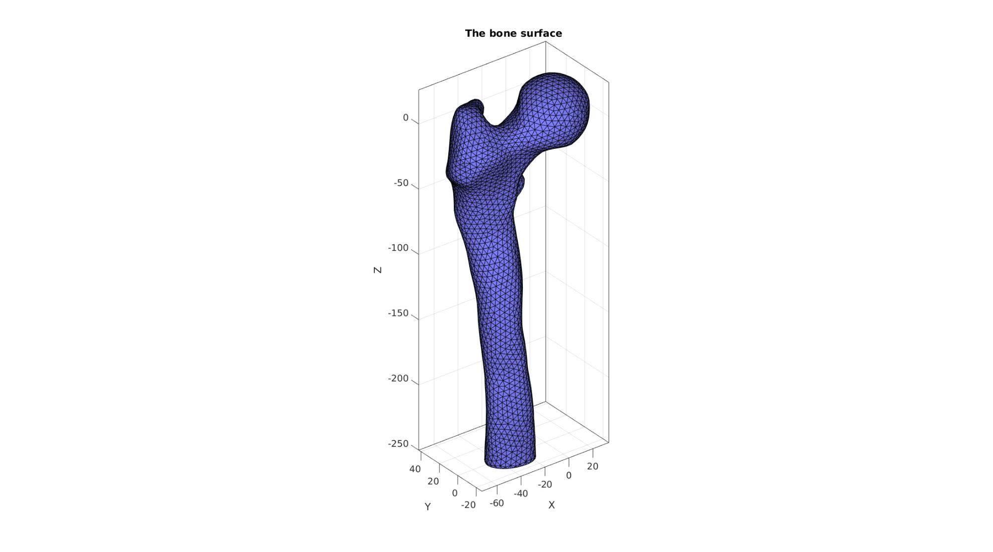
Visualize cut surface

cFigure; hold on;
title('The bone surface');
gpatch(F_bone,V_bone,'bw','k',1);
axisGeom;
camlight headlight;
gdrawnow;

Cut femoral head off

%Set-up orientation and location of cutting plane
n=vecnormalize([0 0 1]); %Normal direction to plane
Q1=euler2DCM([0 -(63/180)*pi 0]);
Q2=euler2DCM([0 0 (32/180)*pi]);
Q=Q1*Q2;
n=n*Q;
P_cut=[0 0 0]-n*stemCut; %Point on plane

%Slicing surface
[Fc,Vc,Cc,logicSide,~]=triSurfSlice(F_bone,V_bone,C_bone,P_cut,n,snapTolerance);

%Compose isolated cut geometry and boundary curves
[F_bone_cut,V_bone_cut]=patchCleanUnused(Fc(logicSide,:),Vc);
C_bone_cut=Cc(logicSide);

Eb=patchBoundary(F_bone_cut);
indCutCurve=edgeListToCurve(Eb);
indCutCurve=indCutCurve(1:end-1);

%Smoothing cut
logicTouch=any(ismember(F_bone_cut,indCutCurve),2);
indTouch=unique(F_bone_cut(logicTouch,:));
logicTouch=any(ismember(F_bone_cut,indTouch),2);
indRigid=unique(F_bone_cut(~logicTouch,:));
indRigid=unique([indRigid(:);indCutCurve(:)]);

clear cparSmooth
cparSmooth.n=numSmoothStepsCutFemur;
cparSmooth.RigidConstraints=indRigid;
[V_bone_cut]=patchSmooth(F_bone_cut,V_bone_cut,[],cparSmooth);

clear cparSmooth
cparSmooth.n=numSmoothStepsCutFemur;
[VEb]=patchSmooth(Eb,V_bone_cut,[],cparSmooth);
V_bone_cut(indCutCurve,:)=VEb(indCutCurve,:);

%Get curve points and centre coordinate
V_bone_cut_curve=V_bone_cut(indCutCurve,:);
PA=mean(V_bone_cut_curve,1); %Mean of cut curve (middle of cut)

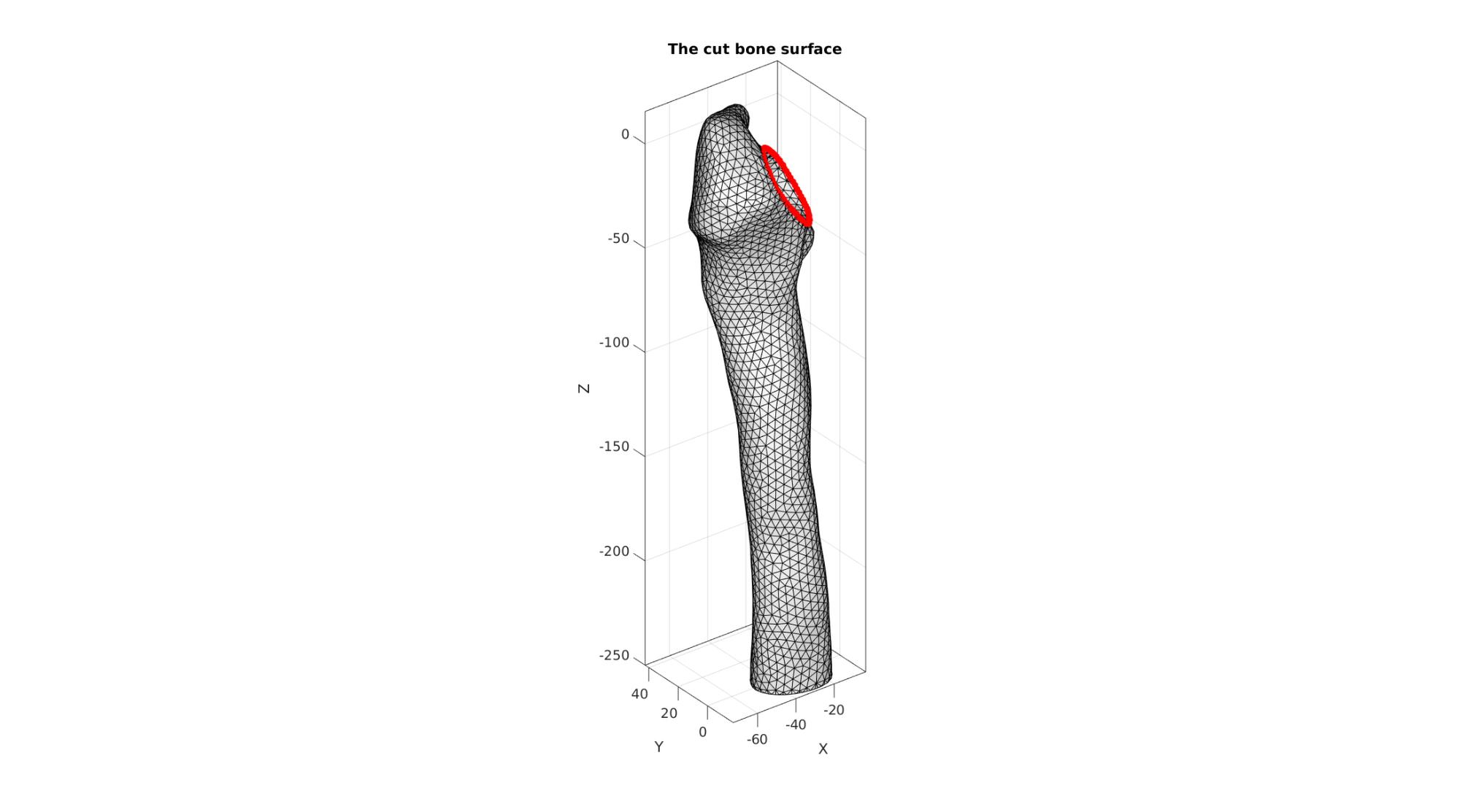
Visualize cut surface

cFigure; hold on;
title('The cut bone surface');
gpatch(F_bone_cut,V_bone_cut,'w','k',1);
plotV(V_bone_cut_curve,'r.-','MarkerSize',25,'LineWidth',3)
axisGeom;
camlight headlight;
gdrawnow;

Add inner bone surface for implant to rest on (will attach to collar)

%Define collar curve
V_collar_1=V_bone_cut_curve;
V_collar_1=V_collar_1-PA;

d=sqrt(sum(V_collar_1.^2,2));
shrinkFactor=(min(d(:))-implantOffsetCollar)./min(d(:));
V_collar_1=V_collar_1.*shrinkFactor;
V_collar_1=V_collar_1+PA;
V_collar_1=evenlySpaceCurve(V_collar_1,pointSpacing,'pchip',1);

% Mesh cut bone top (space between collar curve and bone cut curve)
[F_bone_top,V_bone_top]=regionTriMesh3D({V_bone_cut_curve,V_collar_1},[],0,'linear');
nTop=mean(patchNormal(F_bone_top,V_bone_top),1);
if dot(nTop,n)<0
    F_bone_top=fliplr(F_bone_top);
end

% Join and merge geometry
[F_bone_cut,V_bone_cut,C_bone_cut]=joinElementSets({F_bone_cut,F_bone_top},{V_bone_cut,V_bone_top},{C_bone_cut,max(C_bone_cut(:))+ones(size(F_bone_top,1),1)});
[F_bone_cut,V_bone_cut]=mergeVertices(F_bone_cut,V_bone_cut);

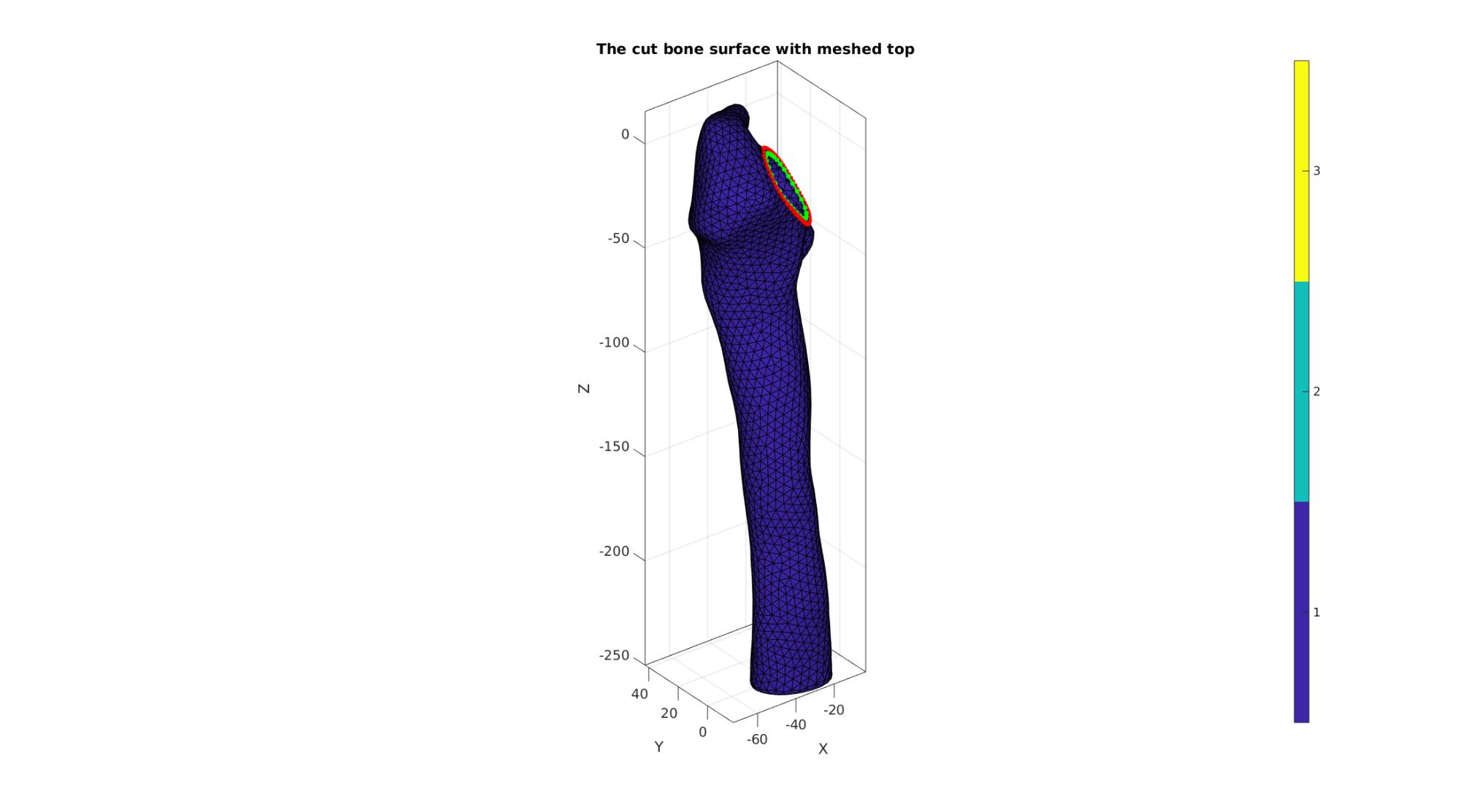
Visualize bone with meshed top

cFigure; hold on;
title('The cut bone surface with meshed top');
gpatch(F_bone_cut,V_bone_cut,C_bone_cut,'k',1);

plotV(V_bone_cut_curve,'r.-','MarkerSize',15,'LineWidth',2)
plotV(V_collar_1,'g.-','MarkerSize',15,'LineWidth',2)
axisGeom; icolorbar;
camlight headlight;
gdrawnow;

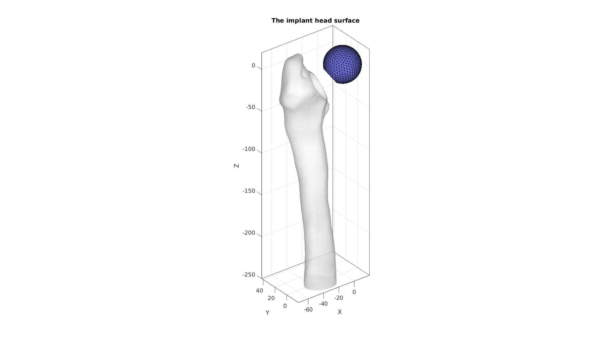
Create implant spherical head

% Create sphere use will loop to define increasingly fine sphere
% triangulations untill the point spacing of the sphere is smaller or equal
% to the bone point spacing.

nRef=1;
while 1
    [F_head,V_head]=geoSphere(nRef,implantHeadRadius);
    pointSpacingNow=mean(patchEdgeLengths(F_head,V_head));
    if pointSpacingNow<=pointSpacing
        break
    else
        nRef=nRef+1;
    end
end

Cutting the sphere

% Define ball cutting coordinate
xc=cos(asin(implantStickRadius/implantHeadRadius))*implantHeadRadius;

logicRight=V_head(:,1)>xc;
logicCut=any(logicRight(F_head),2);
logicCut=triSurfLogicSharpFix(F_head,logicCut,3);
F_head=F_head(~logicCut,:);
[F_head,V_head]=patchCleanUnused(F_head,V_head);
Eb_head=patchBoundary(F_head);
indB=unique(Eb_head(:));
[T,P,R] = cart2sph(V_head(:,2),V_head(:,3),V_head(:,1));
P(indB)=atan2(xc,implantHeadRadius*sin(acos(xc./implantHeadRadius)));
[V_head(:,2),V_head(:,3),V_head(:,1)] = sph2cart(T,P,R);

indHeadHole=edgeListToCurve(Eb_head);
indHeadHole=indHeadHole(1:end-1);

pointSpacingHead=mean(sqrt(sum(diff(V_head(indHeadHole,:),1,1).^2,2)));

%Reorient ball
nd=vecnormalize(-PA); %Vector pointing to mean of cut curve
Q=vecPair2Rot(nd,[0 0 1]); %Rotation matrix for ball
Q3=euler2DCM([0 -0.5*pi 0]);
V_head=V_head*Q3;
V_head=V_head*Q;

Visualize head

cFigure; hold on;
title('The implant head surface');
gpatch(F_bone_cut,V_bone_cut,'w','none',0.5);
gpatch(F_head,V_head,'bw','k',1);
axisGeom; camlight headlight;
gdrawnow;

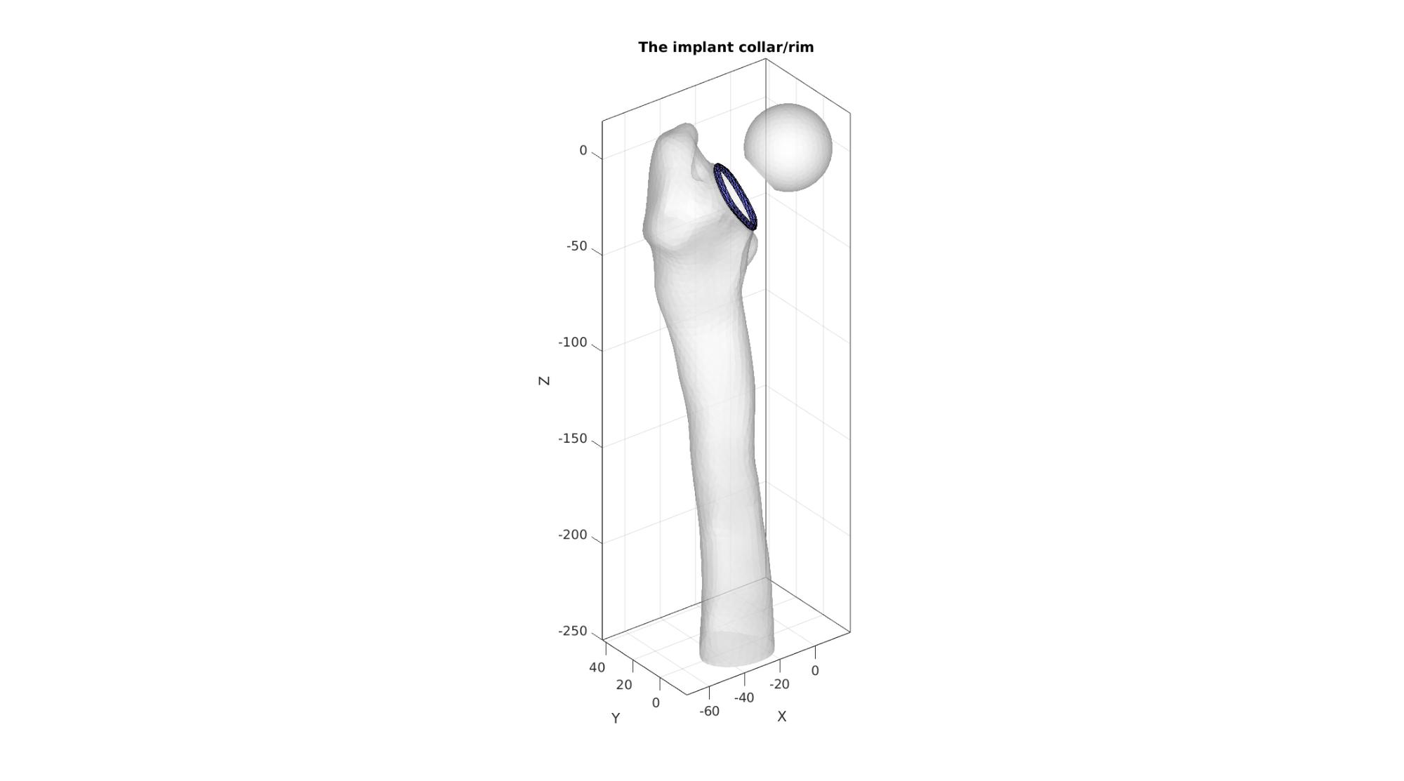
Build colar

%Create color offset curve
V_colarTop=V_collar_1;
ve=[V_colarTop(2:end,:); V_colarTop(1,:)]-V_colarTop;

vd=vecnormalize(cross(n(ones(size(ve,1),1),:),ve));
% vn2(:,1)=vn2(:,1)+collarThickness.*n;
V_colarTop=V_colarTop+implantCollarThickness.*n;

nc=ceil((pi*implantCollarThickness/2)/pointSpacingHead);
if nc<4
    nc=4;
end
vc=linspacen(V_collar_1,V_colarTop,nc);
X=squeeze(vc(:,1,:));
Y=squeeze(vc(:,2,:));
Z=squeeze(vc(:,3,:));
t=repmat(linspace(-1,1,nc),size(Z,1),1);
a=acos(t);
X=X+implantCollarThickness/2.*sin(a).*repmat(vd(:,1),1,nc);
Y=Y+implantCollarThickness/2.*sin(a).*repmat(vd(:,2),1,nc);
Z=Z+implantCollarThickness/2.*sin(a).*repmat(vd(:,3),1,nc);

[F_collar,V_collar]=grid2patch(X,Y,Z,[],[1 0 0]);
[F_collar,V_collar]=quad2tri(F_collar,V_collar,'a');

indTopCollar=size(V_collar,1)+1-size(V_collar_1,1):size(V_collar,1);
Eb_collar=[indTopCollar(:) [indTopCollar(2:end)'; indTopCollar(1)]];

Visualize collar

cFigure; hold on;
title('The implant collar/rim');
gpatch(F_bone_cut,V_bone_cut,'w','none',0.5);
gpatch(F_head,V_head,'w','none',0.5);
gpatch(F_collar,V_collar,'bw','k',1);
axisGeom; camlight headlight;
gdrawnow;

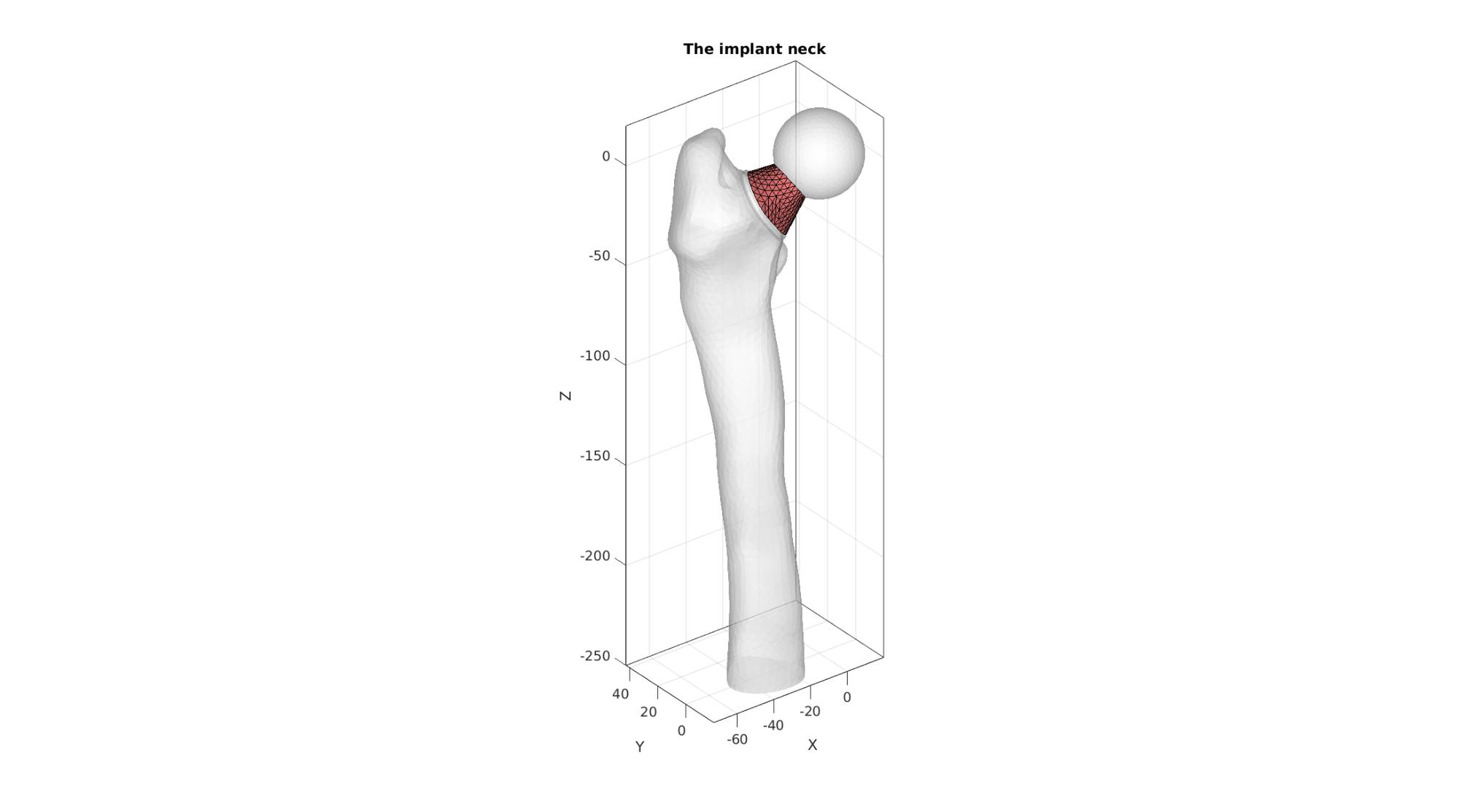
Build neck

if size(Eb_head,1)<size(Eb_collar,1)
    numEdgesNeeded=size(Eb_collar,1);
    [F_head,V_head,Eb_head,~]=triSurfSplitBoundary(F_head,V_head,Eb_head,numEdgesNeeded,[]);
elseif size(Eb_collar,1)<size(Eb_head,1)
    numEdgesNeeded=size(Eb_head,1);
    [F_collar,V_collar,Eb_collar,~]=triSurfSplitBoundary(F_collar,V_collar,Eb_collar,numEdgesNeeded,[]);
end
indTopCollar=edgeListToCurve(Eb_collar); indTopCollar=indTopCollar(1:end-1);
indHeadHole=edgeListToCurve(Eb_head); indHeadHole=indHeadHole(1:end-1);

[~,indStart]=minDist(V_collar(indTopCollar(1),:),V_head(indHeadHole,:));

if indStart>1
    indHeadHole=[indHeadHole(indStart:end) indHeadHole(1:indStart-1)];
end

d1=sum((V_head(indHeadHole,:)-V_collar(indTopCollar,:)).^2,2);
d2=sum((V_head(indHeadHole,:)-V_collar(flip(indTopCollar),:)).^2,2);
if max(d2(:))<max(d1(:))
    indTopCollar=flip(indTopCollar);
end

cParLoft.closeLoopOpt=1;
cParLoft.patchType='tri_slash';
[F_neck,V_neck,indNeckStart,indNeckEnd]=polyLoftLinear(V_collar(indTopCollar,:),V_head(indHeadHole,:),cParLoft);

Visualize collar

cFigure; hold on;
title('The implant neck');
gpatch(F_bone_cut,V_bone_cut,'w','none',0.5);
gpatch(F_head,V_head,'w','none',0.5);
gpatch(F_collar,V_collar,'w','none',0.5);
gpatch(F_neck,V_neck,'rw','k',1);
axisGeom; camlight headlight;
gdrawnow;

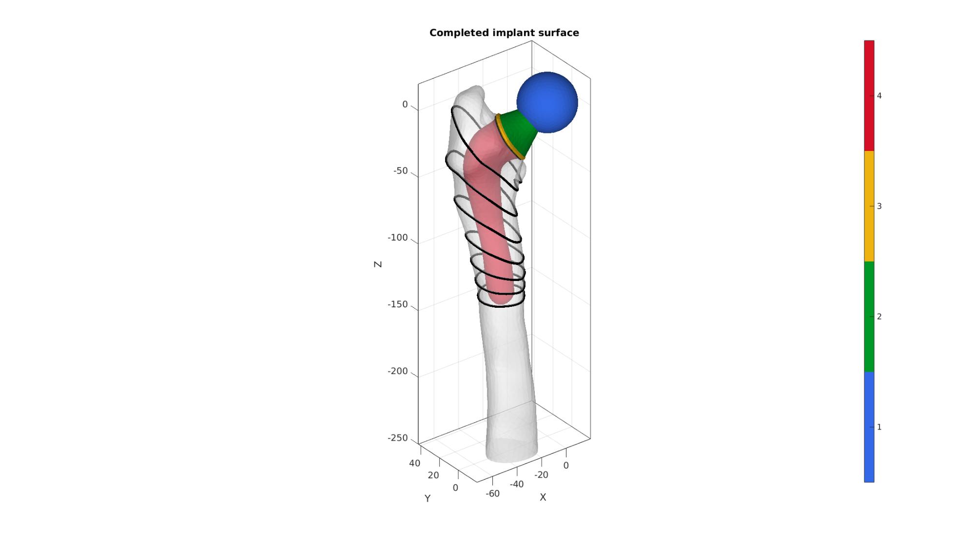
Define shaft

%Find lowest point on collar curve
[~,indMin]=min(V_collar_1(:,3));
PB=V_collar_1(indMin,:);

%Define a normalized vector pointing from PA to PB
m=vecnormalize(PB-PA);

%Define based point for slicing
f=shaftDepthFromHead./abs(m(3));
P=PA+f*m;

%Define normal directions for slicing (go linearly from n to z-dir)
nn=linspacen(n,[0 0 1],numLoftGuideSlicesShaft)';


numPointsRadial=size(V_collar_1,1);
Vp=V_collar_1;
FL=[];
VL=Vp;
[~,indStart]=max(VL(:,1));
if indStart>1
    VL=[VL(indStart:end,:); VL(1:indStart-1,:)];
end
R1=vecPair2Rot(n,[0 0 1]);
e=[(1:numPointsRadial)' [(2:numPointsRadial)';1]];
V_start=VL(1,:);
t=linspace(0,2*pi,numPointsRadial+1); t=t(1:end-1);
VC=cell(numLoftGuideSlicesShaft,1);
VC{1}=V_collar_1;
for q=2:1:numLoftGuideSlicesShaft

    Rn=vecPair2Rot(nn(q,:),[0 0 1]);

    [~,Vqc,~,~,Ebc]=triSurfSlice(F_bone,V_bone,[],P,nn(q,:),snapTolerance);
    indCutCurveNow=edgeListToCurve(Ebc);
    indCutCurveNow=indCutCurveNow(1:end-1);
    P2=mean(Vqc(indCutCurveNow,:),1);

    if P2(3)>-50
        Vp=V_collar_1-PA;
        Vp=Vp*R1';
        Vp=Vp*Rn;
    else
        Vp=Vqc(indCutCurveNow,:);
        Vp=Vp-P2;
        d=sqrt(sum(Vp.^2,2));
        shrinkFactor=(min(d(:))-implantOffset)./min(d(:));
        Vp=Vp.*shrinkFactor;
    end

    Vp=Vp+P2;
    Vp=evenlySampleCurve(Vp,numPointsRadial,0.01,1);

    [~,indStart]=max(Vp(:,1));
    if indStart>1
        Vp=[Vp(indStart:end,:); Vp(1:indStart-1,:)];
    end

    f=[e+(q-2)*numPointsRadial fliplr(e)+(q-1)*numPointsRadial];

    FL=[FL;f];
    VL=[VL;Vp];

    V_start=Vp(1,:);
    VC{q}=Vqc(indCutCurveNow,:);
end

[Fe,Ve]=regionTriMesh3D({Vp},[],0,'linear');
ne=mean(patchNormal(Fe,Ve),1);
if dot(ne,[0 0 1])>0
    Fe=fliplr(Fe);
end
d=minDist(Ve,Vp);
r=max(d(:));
d=d./max(d(:));
a=acos(1-d);
Ve(:,3)=Ve(:,3)-r*sin(a);
[FL,VL]=subQuad(FL,VL,3,3);
[FL,VL]=quad2tri(FL,VL,'a');

[FL,VL]=joinElementSets({FL,Fe},{VL,Ve});
[FL,VL]=mergeVertices(FL,VL);
Eb=patchBoundary(FL);

cparSmooth.n=numSmoothStepsShaft;
% cPar.Method='HC';
cparSmooth.RigidConstraints=unique(Eb(:));
VL=patchSmooth(FL,VL,[],cparSmooth);

% Join and merge surfaces
[F_implant,V_implant,C_implant]=joinElementSets({F_head,F_neck,F_collar,FL},{V_head,V_neck,V_collar,VL});
[F_implant,V_implant]=mergeVertices(F_implant,V_implant);

Visualize implant

cFigure; hold on;
title('Completed implant surface');
gpatch(F_bone_cut,V_bone_cut,'w','none',0.5);
gpatch(F_implant,V_implant,C_implant,'none',1);

for q=1:1:numLoftGuideSlicesShaft
    Vpp=VC{q};
    plotV(Vpp([1:size(Vpp,1) 1],:),'k-','LineWidth',4);
end

axisGeom; camlight headlight;
colormap(gjet(250)); icolorbar;
gdrawnow;

Join bone and implant surfaces

[F,V,C]=joinElementSets({F_bone_cut,F_implant},{V_bone_cut,V_implant},{C_bone_cut,C_implant+max(C_bone_cut(:))});
[F,V]=mergeVertices(F,V);

Visualized merged set

cFigure; hold on;
gpatch(F,V,C,'none',0.5);
axisGeom; camlight headlight;
colormap(gjet(250)); icolorbar;
gdrawnow;

Create tetrahedral elements for both regions

Define interior points

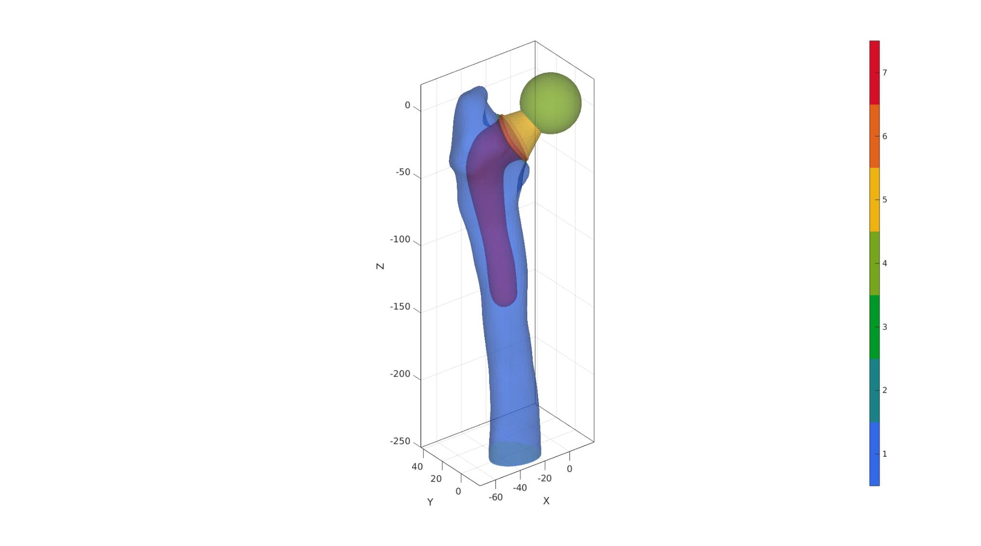
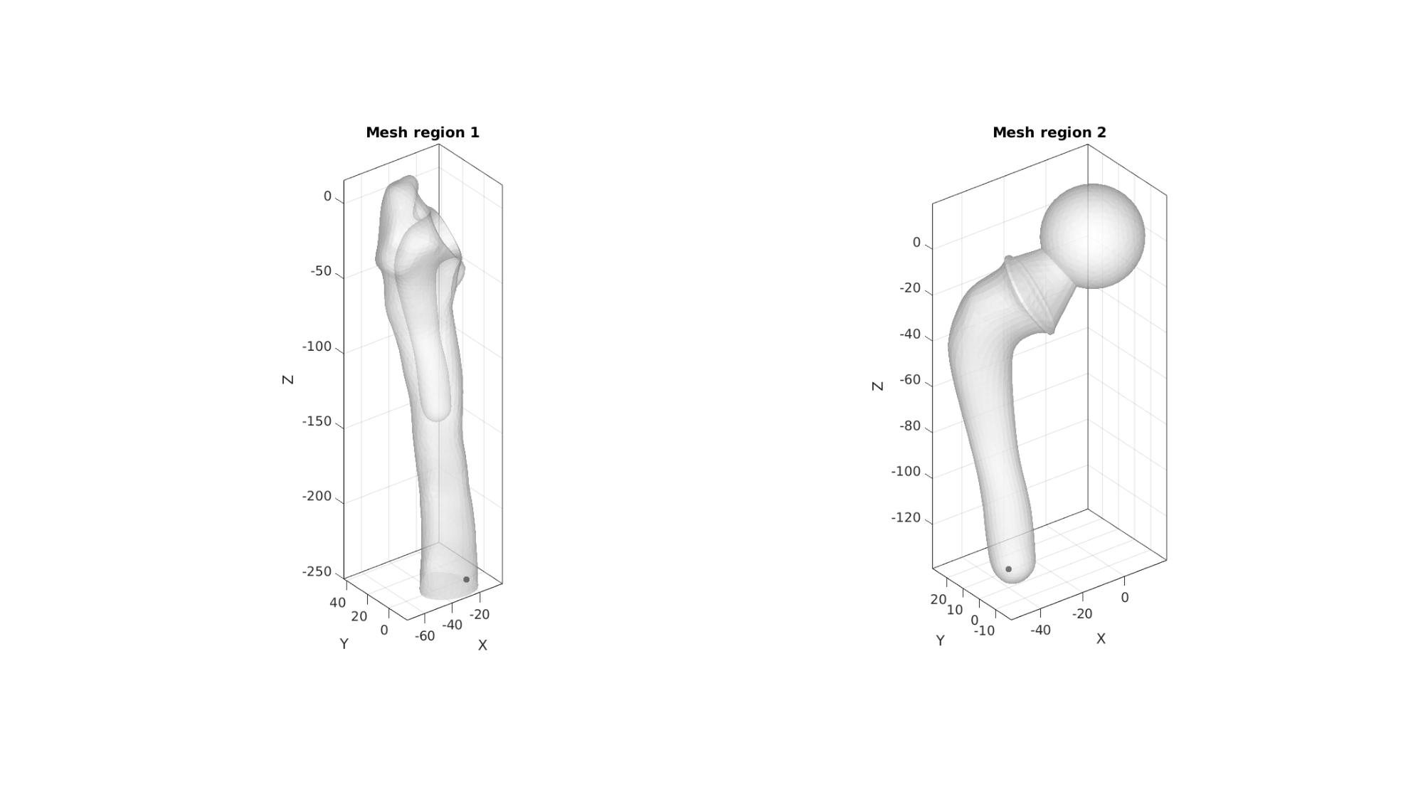
logicRegion1=ismember(C,[1 2 3 7]); %Bone region is defined by bone+shaft surfaces
V_region1=getInnerPoint(F(logicRegion1,:),V);

logicRegion2=ismember(C,4:7); %Logic for implant faces
V_region2=getInnerPoint(F(logicRegion2,:),V);

V_regions=[V_region1; V_region2];

Visualize mesh regions and interior points

cFigure;
subplot(1,2,1); hold on;
title('Mesh region 1');
gpatch(F(logicRegion1,:),V,'w','none',0.5);
plotV(V_region1,'k.','MarkerSize',25);
axisGeom; camlight headlight;

subplot(1,2,2); hold on;
title('Mesh region 2');
gpatch(F(logicRegion2,:),V,'w','none',0.5);
plotV(V_region2,'k.','MarkerSize',25);
axisGeom; camlight headlight;

gdrawnow;

Mesh using TetGen

regionTetVolumes=volumeFactors.*tetVolMeanEst(F,V);

%Create tetgen input structure
inputStruct.stringOpt='-pq1.2AaY'; %Options for tetgen
inputStruct.Faces=F; %Boundary faces
inputStruct.Nodes=V; %Nodes of boundary
inputStruct.faceBoundaryMarker=C;
inputStruct.regionPoints=V_regions; %Interior points for regions
inputStruct.holePoints=[]; %Interior points for holes
inputStruct.regionA=regionTetVolumes; %Desired tetrahedral volume for each region

% Mesh model using tetrahedral elements using tetGen
[meshOutput]=runTetGen(inputStruct); %Run tetGen

 
%%%%%%%%%%%%%%%%%%%%%%%%%%%%%%%%%%%%%%%%%%%%%
--- TETGEN Tetrahedral meshing --- 29-May-2023 10:39:08
 
%%%%%%%%%%%%%%%%%%%%%%%%%%%%%%%%%%%%%%%%%%%%%
--- Writing SMESH file --- 29-May-2023 10:39:08
----> Adding node field
----> Adding facet field
----> Adding holes specification
----> Adding region specification
--- Done --- 29-May-2023 10:39:08
--- Running TetGen to mesh input boundary--- 29-May-2023 10:39:08
Opening /home/kevin/DATA/Code/matlab/GIBBON/data/temp/temp.smesh.
Delaunizing vertices...
Delaunay seconds:  0.020498
Creating surface mesh ...
Surface mesh seconds:  0.004431
Recovering boundaries...
Boundary recovery seconds:  0.008259
Removing exterior tetrahedra ...
Spreading region attributes.
Exterior tets removal seconds:  0.003486
Recovering Delaunayness...
Delaunay recovery seconds:  0.006234
Refining mesh...
  6679 insertions, added 5728 points, 197840 tetrahedra in queue.
  2224 insertions, added 1564 points, 211485 tetrahedra in queue.
  2964 insertions, added 1320 points, 85537 tetrahedra in queue.
Refinement seconds:  0.131803
Smoothing vertices...
Mesh smoothing seconds:  0.223018
Improving mesh...
Mesh improvement seconds:  0.008581

Writing /home/kevin/DATA/Code/matlab/GIBBON/data/temp/temp.1.node.
Writing /home/kevin/DATA/Code/matlab/GIBBON/data/temp/temp.1.ele.
Writing /home/kevin/DATA/Code/matlab/GIBBON/data/temp/temp.1.face.
Writing /home/kevin/DATA/Code/matlab/GIBBON/data/temp/temp.1.edge.

Output seconds:  0.032528
Total running seconds:  0.439064

Statistics:

  Input points: 5011
  Input facets: 10046
  Input segments: 15054
  Input holes: 0
  Input regions: 2

  Mesh points: 13953
  Mesh tetrahedra: 75470
  Mesh faces: 154199
  Mesh faces on exterior boundary: 6518
  Mesh faces on input facets: 10046
  Mesh edges on input segments: 15054
  Steiner points inside domain: 8942

--- Done --- 29-May-2023 10:39:09
 
%%%%%%%%%%%%%%%%%%%%%%%%%%%%%%%%%%%%%%%%%%%%%
--- Importing TetGen files --- 29-May-2023 10:39:09
--- Done --- 29-May-2023 10:39:09

Access mesh output structure

E=meshOutput.elements; %The elements
V=meshOutput.nodes; %The vertices or nodes
CE=meshOutput.elementMaterialID; %Element material or region id
Fb=meshOutput.facesBoundary; %The boundary faces
Cb=meshOutput.boundaryMarker; %The boundary markers

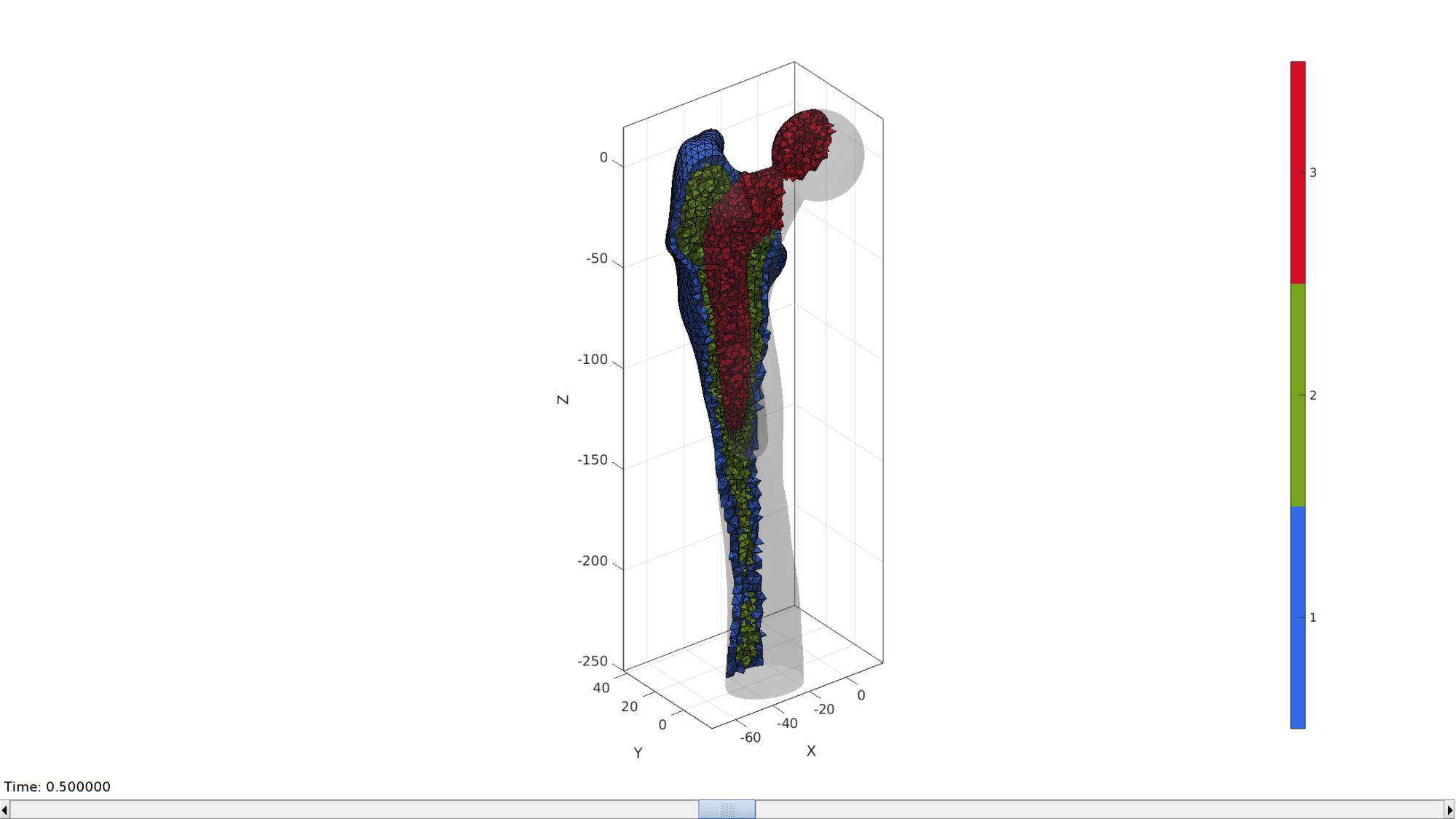
Define material regions in bone

logicImplantElements=CE==-3;

indBoundary=unique(Fb(Cb==1,:));
DE=minDist(V,V(indBoundary,:));
logicCorticalNodes=DE<=corticalThickness;
logicCorticalElements=any(logicCorticalNodes(E),2) & ~logicImplantElements;
logicCancellousElements=~logicCorticalElements & ~logicImplantElements;

E1=E(logicCorticalElements,:);
E2=E(logicCancellousElements,:);
E3=E(logicImplantElements,:);
E=[E1;E2;E3];

elementMaterialID=[ones(size(E1,1),1);2*ones(size(E2,1),1);3*ones(size(E3,1),1)];
logicBoneElements=ismember(elementMaterialID,[1 2]);
E_12=E(logicBoneElements,:); %Only bone elements
VE_12=patchCentre(E_12,V); %Centre coordinates for bone elements

meshOutput.elements=E;
meshOutput.elementMaterialID=elementMaterialID;

Visualizing solid mesh

hFig=cFigure; hold on;
optionStruct.hFig=hFig;
meshView(meshOutput,optionStruct);
axisGeom;
drawnow;

Load SED data from non-implant model and access SED interpolation function

if skipCompare==0 %Load data without implant
    outputStruct=load(loadName_SED);
    Fb_no_implant = outputStruct.boundaryFaces;
    V_no_implant = outputStruct.nodes;
    interpFuncEnergy=outputStruct.interpFuncEnergy; % Interpolation function
end

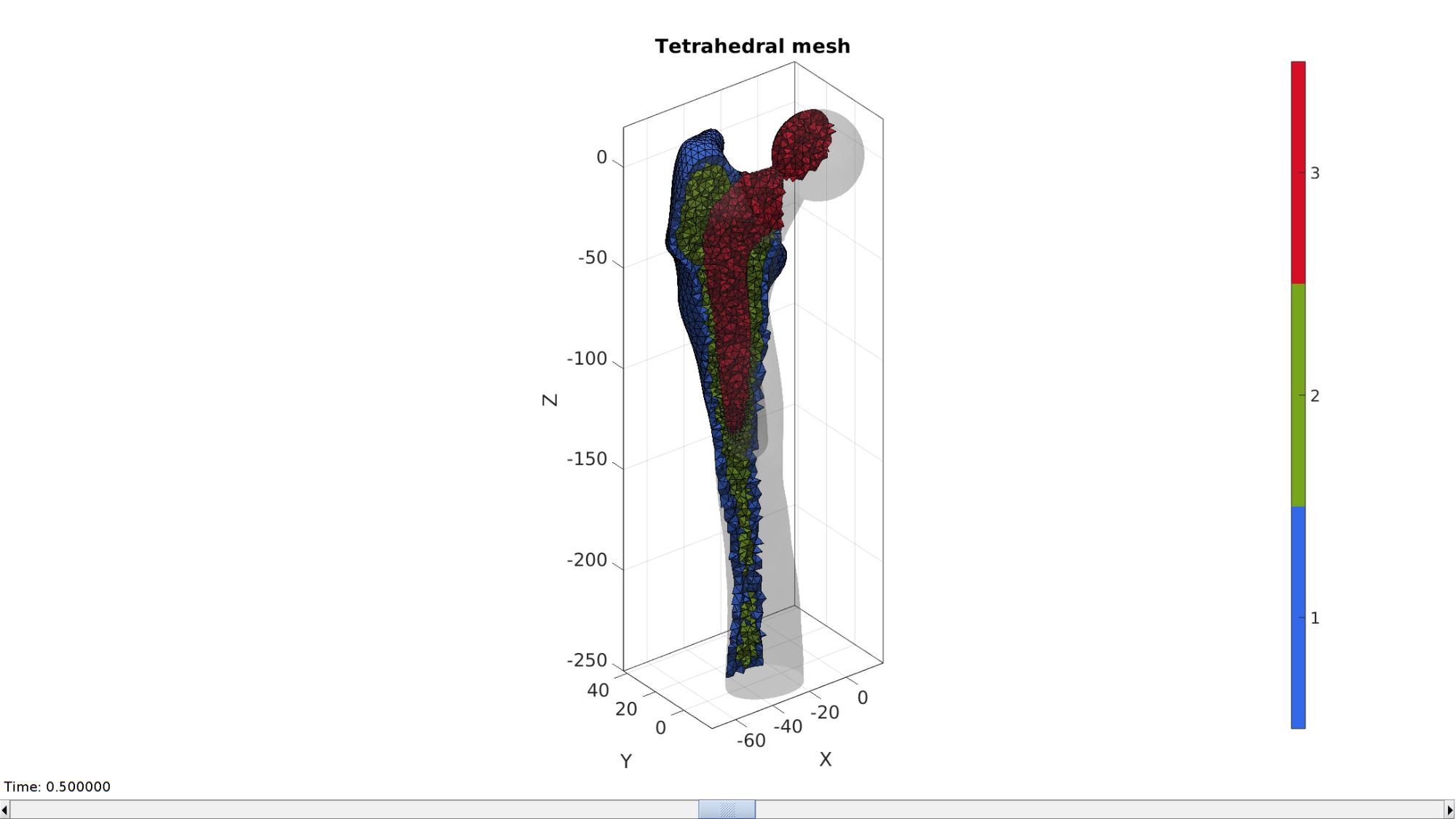
Visualize solid mesh

hf=cFigure; hold on;
title('Tetrahedral mesh','FontSize',fontSize);
% Visualizing using |meshView|
optionStruct.hFig=hf;
meshView(meshOutput,optionStruct);

axisGeom(gca,fontSize);
gdrawnow;

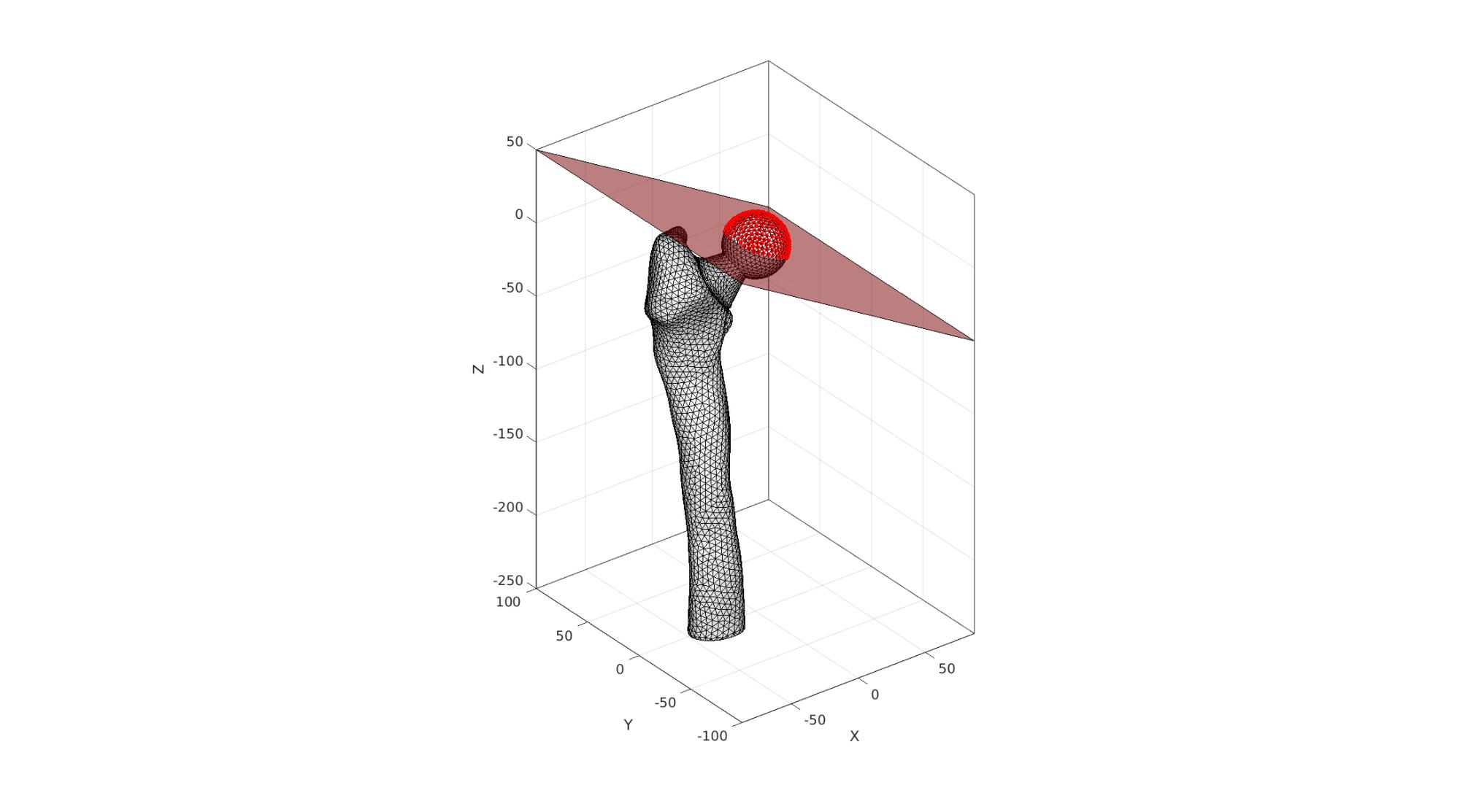
Find femoral head

w=100;
f=[1 2 3 4];
v=w*[-1 -1 0; -1 1 0; 1 1 0; 1 -1 0];

p=[0 0 0];
Q=euler2DCM([0 (150/180)*pi 0]);
v=v*Q;
v=v+p;

Vr=V*Q';
Vr=Vr+p;
logicHeadNodes=Vr(:,3)<0;
logicHeadFaces=all(logicHeadNodes(Fb),2);
bcPrescribeList_head=unique(Fb(logicHeadFaces,:));

Visualize femoral head nodes for prescribed force boundary conditions

cFigure;
hold on;
gpatch(Fb,V,'w','k',1);
gpatch(f,v,'r','k',0.5);
plotV(V(bcPrescribeList_head,:),'r.','markerSize',15)
axisGeom; camlight headlight;
drawnow;

Work out force distribution on femoral head surface nodes

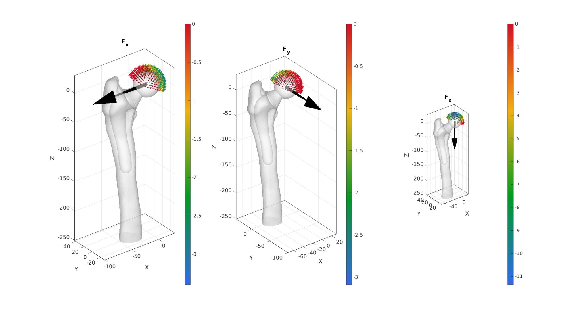
This is based on surface normal directions. Forces are assumed to only be able to act in a compressive sense on the bone.

[~,~,N]=patchNormal(fliplr(Fb),V); %Nodal normal directions

FX=[forceTotal(1) 0 0]; %X force vector
FY=[0 forceTotal(2) 0]; %Y force vector
FZ=[0 0 forceTotal(3)]; %Z force vector

wx=dot(N(bcPrescribeList_head,:),FX(ones(numel(bcPrescribeList_head),1),:),2);
wy=dot(N(bcPrescribeList_head,:),FY(ones(numel(bcPrescribeList_head),1),:),2);
wz=dot(N(bcPrescribeList_head,:),FZ(ones(numel(bcPrescribeList_head),1),:),2);

%Force zero
wx(wx>0)=0; wy(wy>0)=0; wz(wz>0)=0;

force_X=forceTotal(1).*ones(numel(bcPrescribeList_head),1).*wx;
force_Y=forceTotal(2).*ones(numel(bcPrescribeList_head),1).*wy;
force_Z=forceTotal(3).*ones(numel(bcPrescribeList_head),1).*wz;

force_X=force_X./sum(force_X(:)); %sum now equal to 1
force_X=force_X.*forceTotal(1); %sum now equal to desired

force_Y=force_Y./sum(force_Y(:)); %sum now equal to 1
force_Y=force_Y.*forceTotal(2); %sum now equal to desired

force_Z=force_Z./sum(force_Z(:)); %sum now equal to 1
force_Z=force_Z.*forceTotal(3); %sum now equal to desired

force_head=[force_X(:) force_Y(:) force_Z(:)];

cFigure;
subplot(1,3,1);hold on;
title('F_x');
gpatch(Fb,V,'w','none',0.5);
quiverVec([0 0 0],FX,100,'k');
% scatterV(V(indicesHeadNodes,:),15)
quiverVec(V(bcPrescribeList_head,:),N(bcPrescribeList_head,:),10,force_X);
axisGeom; camlight headlight;
colormap(gca,gjet(250)); colorbar;

subplot(1,3,2);hold on;
title('F_y');
gpatch(Fb,V,'w','none',0.5);
quiverVec([0 0 0],FY,100,'k');
% scatterV(V(indicesHeadNodes,:),15)
quiverVec(V(bcPrescribeList_head,:),N(bcPrescribeList_head,:),10,force_Y);
axisGeom; camlight headlight;
colormap(gca,gjet(250)); colorbar;

subplot(1,3,3);hold on;
title('F_z');
gpatch(Fb,V,'w','none',0.5);
quiverVec([0 0 0],FZ,100,'k');
% scatterV(V(indicesHeadNodes,:),15)
quiverVec(V(bcPrescribeList_head,:),N(bcPrescribeList_head,:),10,force_Z);
axisGeom; camlight headlight;
colormap(gca,gjet(250)); colorbar;

drawnow;

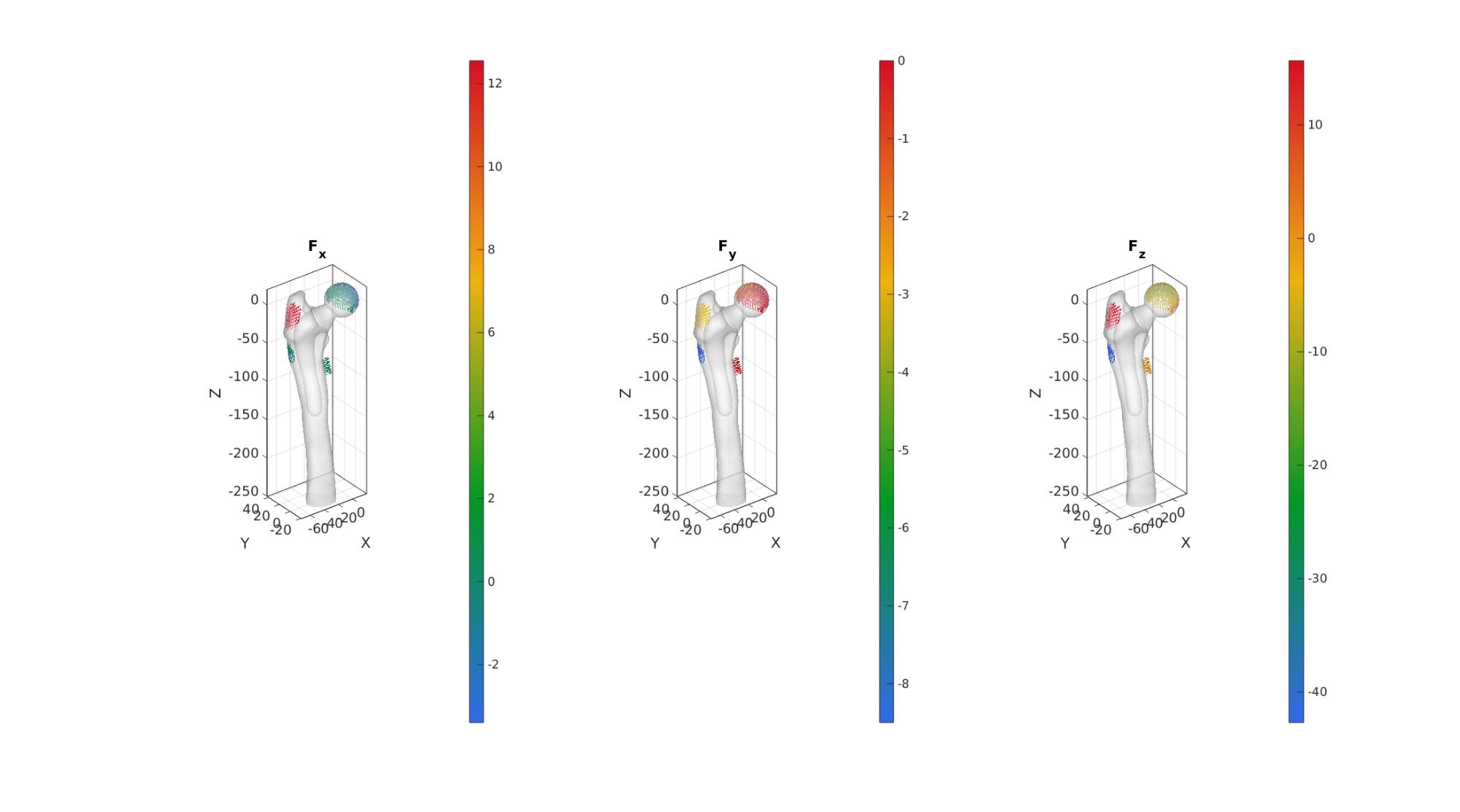
Marking muscle locations

P_abductor_find = [-69.771045288206111 8.185179717034659 -5.575329878303917]; %Coordinate at centre of muscle attachment
[~,indAbductor]=minDist(P_abductor_find,V); %Node number of point at centre of attachment
dAbductor=meshDistMarch(Fb,V,indAbductor); %Distance (on mesh) from attachement centre
bcPrescibeList_abductor=find(dAbductor<=distanceMuscleAttachAbductor); %Node numbers for attachment site

P_VastusLateralis_find = [-58.763839901506827 19.145444610053566 -51.005278396808819]; %Coordinate at centre of muscle attachment
[~,indVastusLateralis]=minDist(P_VastusLateralis_find,V); %Node number of point at centre of attachment
dVastusLateralis=meshDistMarch(Fb,V,indVastusLateralis); %Distance (on mesh) from attachement centre
bcPrescibeList_VastusLateralis=find(dVastusLateralis<=distanceMuscleVastusLateralis); %Node numbers for attachment site


P_VastusMedialis_find = [-18.533631492778085 9.501312355952791 -85.666499329588035]; %Coordinate at centre of muscle attachment
[~,indVastusMedialis]=minDist(P_VastusMedialis_find,V); %Node number of point at centre of attachment
dVastusMedialis=meshDistMarch(Fb,V,indVastusMedialis); %Distance (on mesh) from attachement centre
bcPrescibeList_VastusMedialis=find(dVastusMedialis<=distanceMuscleAttachVastusMedialis); %Node numbers for attachment site

Muscle force definition

forceAbductor_distributed=forceAbductor.*ones(numel(bcPrescibeList_abductor),1)./numel(bcPrescibeList_abductor);

forceVastusLateralis_distributed=forceVastusLateralis.*ones(numel(bcPrescibeList_VastusLateralis),1)./numel(bcPrescibeList_VastusLateralis);

forceVastusMedialis_distributed=forceVastusMedialis.*ones(numel(bcPrescibeList_VastusMedialis),1)./numel(bcPrescibeList_VastusMedialis);

Defining prescribed forces

bcPrescribeList=[bcPrescribeList_head(:);...
                 bcPrescibeList_abductor(:);...
                 bcPrescibeList_VastusLateralis(:);...
                 bcPrescibeList_VastusMedialis(:)];

forceData=[force_head;...
           forceAbductor_distributed;...
           forceVastusLateralis_distributed;...
           forceVastusMedialis_distributed];

cFigure;
subplot(1,3,1);hold on;
title('F_x');
gpatch(Fb,V,'w','none',0.5);
quiverVec(V(bcPrescribeList,:),forceData,10,forceData(:,1));
axisGeom; camlight headlight;
colormap(gca,gjet(250)); colorbar;

subplot(1,3,2);hold on;
title('F_y');
gpatch(Fb,V,'w','none',0.5);
quiverVec(V(bcPrescribeList,:),forceData,10,forceData(:,2));
axisGeom; camlight headlight;
colormap(gca,gjet(250)); colorbar;

subplot(1,3,3);hold on;
title('F_z');
gpatch(Fb,V,'w','none',0.5);

quiverVec(V(bcPrescribeList,:),forceData,10,forceData(:,3));
axisGeom; camlight headlight;
colormap(gca,gjet(250)); colorbar;

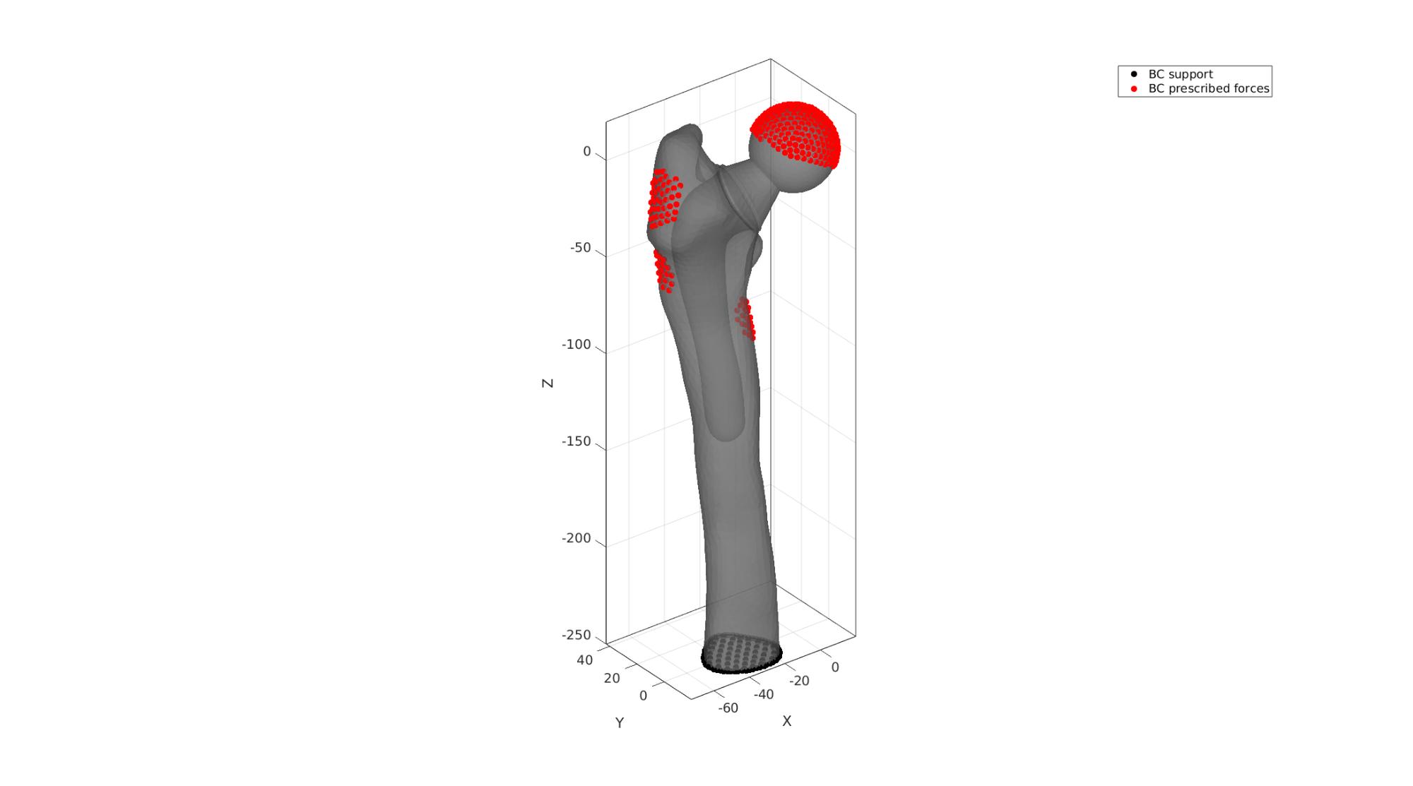
Visualizing boundary conditions

F_bottomSupport=Fb(Cb==2,:);
bcSupportList=unique(F_bottomSupport(:));

cFigure; hold on;
gpatch(Fb,V,'kw','none',0.7);
hl(1)=plotV(V(bcSupportList,:),'k.','MarkerSize',25);
hl(2)=plotV(V(bcPrescribeList,:),'r.','MarkerSize',25);

legend(hl,{'BC support','BC prescribed forces'});
axisGeom;
camlight headlight;
drawnow;

Defining the FEBio input structure

See also febioStructTemplate and febioStruct2xml and the FEBio user manual.

%Get a template with default settings
[febio_spec]=febioStructTemplate;

%febio_spec version
febio_spec.ATTR.version='4.0';

%Module section
febio_spec.Module.ATTR.type='solid';

%Control section
febio_spec.Control.analysis='STATIC';
febio_spec.Control.time_steps=numTimeSteps;
febio_spec.Control.step_size=1/numTimeSteps;
febio_spec.Control.solver.max_refs=max_refs;
febio_spec.Control.solver.qn_method.max_ups=max_ups;
febio_spec.Control.time_stepper.dtmin=dtmin;
febio_spec.Control.time_stepper.dtmax=dtmax;
febio_spec.Control.time_stepper.max_retries=max_retries;
febio_spec.Control.time_stepper.opt_iter=opt_iter;

%Material section
materialName1='Material1';
febio_spec.Material.material{1}.ATTR.name=materialName1;
febio_spec.Material.material{1}.ATTR.type='neo-Hookean';
febio_spec.Material.material{1}.ATTR.id=1;
febio_spec.Material.material{1}.E=E_youngs1;
febio_spec.Material.material{1}.v=nu1;

materialName2='Material2';
febio_spec.Material.material{2}.ATTR.name=materialName2;
febio_spec.Material.material{2}.ATTR.type='neo-Hookean';
febio_spec.Material.material{2}.ATTR.id=2;
febio_spec.Material.material{2}.E=E_youngs2;
febio_spec.Material.material{2}.v=nu2;

materialName3='Material3';
febio_spec.Material.material{3}.ATTR.name=materialName3;
febio_spec.Material.material{3}.ATTR.type='neo-Hookean';
febio_spec.Material.material{3}.ATTR.id=3;
febio_spec.Material.material{3}.E=E_youngs3;
febio_spec.Material.material{3}.v=nu3;

% Mesh section
% -> Nodes
febio_spec.Mesh.Nodes{1}.ATTR.name='Object1'; %The node set name
febio_spec.Mesh.Nodes{1}.node.ATTR.id=(1:size(V,1))'; %The node id's
febio_spec.Mesh.Nodes{1}.node.VAL=V; %The nodel coordinates

% -> Elements
partName1='CorticalBone';
febio_spec.Mesh.Elements{1}.ATTR.name=partName1; %Name of this part
febio_spec.Mesh.Elements{1}.ATTR.type='tet4'; %Element type
febio_spec.Mesh.Elements{1}.elem.ATTR.id=(1:1:size(E1,1))'; %Element id's
febio_spec.Mesh.Elements{1}.elem.VAL=E1; %The element matrix

partName2='CancellousBone';
febio_spec.Mesh.Elements{2}.ATTR.name=partName2; %Name of this part
febio_spec.Mesh.Elements{2}.ATTR.type='tet4'; %Element type
febio_spec.Mesh.Elements{2}.elem.ATTR.id=size(E1,1)+(1:1:size(E2,1))'; %Element id's
febio_spec.Mesh.Elements{2}.elem.VAL=E2; %The element matrix

partName3='Implant';
febio_spec.Mesh.Elements{3}.ATTR.name=partName3; %Name of this part
febio_spec.Mesh.Elements{3}.ATTR.type='tet4'; %Element type
febio_spec.Mesh.Elements{3}.elem.ATTR.id=size(E1,1)+size(E2,1)+(1:1:size(E3,1))'; %Element id's
febio_spec.Mesh.Elements{3}.elem.VAL=E3; %The element matrix

% -> NodeSets
nodeSetName1='bcSupportList';
febio_spec.Mesh.NodeSet{1}.ATTR.name=nodeSetName1;
febio_spec.Mesh.NodeSet{1}.VAL=mrow(bcSupportList);

nodeSetName2='bcPrescribeList';
febio_spec.Mesh.NodeSet{2}.ATTR.name=nodeSetName2;
febio_spec.Mesh.NodeSet{2}.VAL=mrow(bcPrescribeList);

%MeshDomains section
febio_spec.MeshDomains.SolidDomain{1}.ATTR.name=partName1;
febio_spec.MeshDomains.SolidDomain{1}.ATTR.mat=materialName1;

febio_spec.MeshDomains.SolidDomain{2}.ATTR.name=partName2;
febio_spec.MeshDomains.SolidDomain{2}.ATTR.mat=materialName2;

febio_spec.MeshDomains.SolidDomain{3}.ATTR.name=partName3;
febio_spec.MeshDomains.SolidDomain{3}.ATTR.mat=materialName3;

%Boundary condition section
% -> Fix boundary conditions
febio_spec.Boundary.bc{1}.ATTR.name='zero_displacement_xyz';
febio_spec.Boundary.bc{1}.ATTR.type='zero displacement';
febio_spec.Boundary.bc{1}.ATTR.node_set=nodeSetName1;
febio_spec.Boundary.bc{1}.x_dof=1;
febio_spec.Boundary.bc{1}.y_dof=1;
febio_spec.Boundary.bc{1}.z_dof=1;

%MeshData secion
%-> Node data
loadDataName1='nodal_forces';
febio_spec.MeshData.NodeData{1}.ATTR.name=loadDataName1;
febio_spec.MeshData.NodeData{1}.ATTR.node_set=nodeSetName2;
febio_spec.MeshData.NodeData{1}.ATTR.data_type='vec3';
febio_spec.MeshData.NodeData{1}.node.ATTR.lid=(1:1:numel(bcPrescribeList))';
febio_spec.MeshData.NodeData{1}.node.VAL=forceData;

%Loads section
% -> Prescribed nodal forces
febio_spec.Loads.nodal_load{1}.ATTR.name='PrescribedForce';
febio_spec.Loads.nodal_load{1}.ATTR.type='nodal_force';
febio_spec.Loads.nodal_load{1}.ATTR.node_set=nodeSetName2;
febio_spec.Loads.nodal_load{1}.value.ATTR.lc=1;
febio_spec.Loads.nodal_load{1}.value.ATTR.type='map';
febio_spec.Loads.nodal_load{1}.value.VAL=loadDataName1;

%LoadData section
% -> load_controller
febio_spec.LoadData.load_controller{1}.ATTR.name='LC_1';
febio_spec.LoadData.load_controller{1}.ATTR.id=1;
febio_spec.LoadData.load_controller{1}.ATTR.type='loadcurve';
febio_spec.LoadData.load_controller{1}.interpolate='LINEAR';
%febio_spec.LoadData.load_controller{1}.extend='CONSTANT';
febio_spec.LoadData.load_controller{1}.points.pt.VAL=[0 0; 1 1];

%Output section
% -> log file
febio_spec.Output.logfile.ATTR.file=febioLogFileName;
febio_spec.Output.logfile.node_data{1}.ATTR.file=febioLogFileName_disp;
febio_spec.Output.logfile.node_data{1}.ATTR.data='ux;uy;uz';
febio_spec.Output.logfile.node_data{1}.ATTR.delim=',';

febio_spec.Output.logfile.element_data{1}.ATTR.file=febioLogFileName_stress;
febio_spec.Output.logfile.element_data{1}.ATTR.data='s1;s2;s3';
febio_spec.Output.logfile.element_data{1}.ATTR.delim=',';

febio_spec.Output.logfile.element_data{2}.ATTR.file=febioLogFileName_strainEnergy;
febio_spec.Output.logfile.element_data{2}.ATTR.data='sed';
febio_spec.Output.logfile.element_data{2}.ATTR.delim=',';

% Plotfile section
febio_spec.Output.plotfile.compression=0;

Quick viewing of the FEBio input file structure

The febView function can be used to view the xml structure in a MATLAB figure window.

febView(febio_spec); %Viewing the febio file

Exporting the FEBio input file

Exporting the febio_spec structure to an FEBio input file is done using the febioStruct2xml function.

febioStruct2xml(febio_spec,febioFebFileName); %Exporting to file and domNode

Running the FEBio analysis

To run the analysis defined by the created FEBio input file the runMonitorFEBio function is used. The input for this function is a structure defining job settings e.g. the FEBio input file name. The optional output runFlag informs the user if the analysis was run succesfully.

febioAnalysis.run_filename=febioFebFileName; %The input file name
febioAnalysis.run_logname=febioLogFileName; %The name for the log file
febioAnalysis.disp_on=1; %Display information on the command window
febioAnalysis.runMode=runMode;

[runFlag]=runMonitorFEBio(febioAnalysis);%START FEBio NOW!!!!!!!!

 
%%%%%%%%%%%%%%%%%%%%%%%%%%%%%%%%%%%%%%%%%%%%%%%%%%%%%%%%%%%%%%%%%%%%%%%%%%%
-------->    RUNNING/MONITORING FEBIO JOB    <-------- 29-May-2023 10:39:18
FEBio path: /home/kevin/FEBioStudio/bin/febio4
# Attempt removal of existing log files                29-May-2023 10:39:18
 * Removal succesful                                   29-May-2023 10:39:18
# Attempt removal of existing .xplt files              29-May-2023 10:39:18
 * Removal succesful                                   29-May-2023 10:39:18
# Starting FEBio...                                    29-May-2023 10:39:18
  Max. total analysis time is: Inf s
 * Waiting for log file creation                       29-May-2023 10:39:18
   Max. wait time: 30 s
 * Log file found.                                     29-May-2023 10:39:19
# Parsing log file...                                  29-May-2023 10:39:19
    number of iterations   : 3                         29-May-2023 10:39:22
    number of reformations : 3                         29-May-2023 10:39:22
------- converged at time : 0.1                        29-May-2023 10:39:22
    number of iterations   : 3                         29-May-2023 10:39:22
    number of reformations : 3                         29-May-2023 10:39:22
------- converged at time : 0.2                        29-May-2023 10:39:22
    number of iterations   : 3                         29-May-2023 10:39:25
    number of reformations : 3                         29-May-2023 10:39:25
------- converged at time : 0.3                        29-May-2023 10:39:25
    number of iterations   : 3                         29-May-2023 10:39:28
    number of reformations : 3                         29-May-2023 10:39:28
------- converged at time : 0.4                        29-May-2023 10:39:28
    number of iterations   : 3                         29-May-2023 10:39:28
    number of reformations : 3                         29-May-2023 10:39:28
------- converged at time : 0.5                        29-May-2023 10:39:28
    number of iterations   : 3                         29-May-2023 10:39:32
    number of reformations : 3                         29-May-2023 10:39:32
------- converged at time : 0.6                        29-May-2023 10:39:32
    number of iterations   : 3                         29-May-2023 10:39:32
    number of reformations : 3                         29-May-2023 10:39:32
------- converged at time : 0.7                        29-May-2023 10:39:32
    number of iterations   : 3                         29-May-2023 10:39:34
    number of reformations : 3                         29-May-2023 10:39:34
------- converged at time : 0.8                        29-May-2023 10:39:34
    number of iterations   : 3                         29-May-2023 10:39:34
    number of reformations : 3                         29-May-2023 10:39:34
------- converged at time : 0.9                        29-May-2023 10:39:34
    number of iterations   : 3                         29-May-2023 10:39:36
    number of reformations : 3                         29-May-2023 10:39:36
------- converged at time : 1                          29-May-2023 10:39:36
 Elapsed time : 0:00:17                                29-May-2023 10:39:36
 N O R M A L   T E R M I N A T I O N
# Done                                                 29-May-2023 10:39:36
%%%%%%%%%%%%%%%%%%%%%%%%%%%%%%%%%%%%%%%%%%%%%%%%%%%%%%%%%%%%%%%%%%%%%%%%%%%

Import FEBio results

if runFlag==1 %i.e. a succesful run

Importing nodal displacements from a log file

    dataStruct=importFEBio_logfile(fullfile(savePath,febioLogFileName_disp),0,1);

    %Access data
    N_disp_mat=dataStruct.data; %Displacement
    timeVec=dataStruct.time; %Time

    %Create deformed coordinate set
    V_DEF=N_disp_mat+repmat(V,[1 1 size(N_disp_mat,3)]);

Importing element strain energies from a log file

    dataStruct=importFEBio_logfile(fullfile(savePath,febioLogFileName_strainEnergy),0,1); %Element strain energy

    %Access data
    E_energy=dataStruct.data;

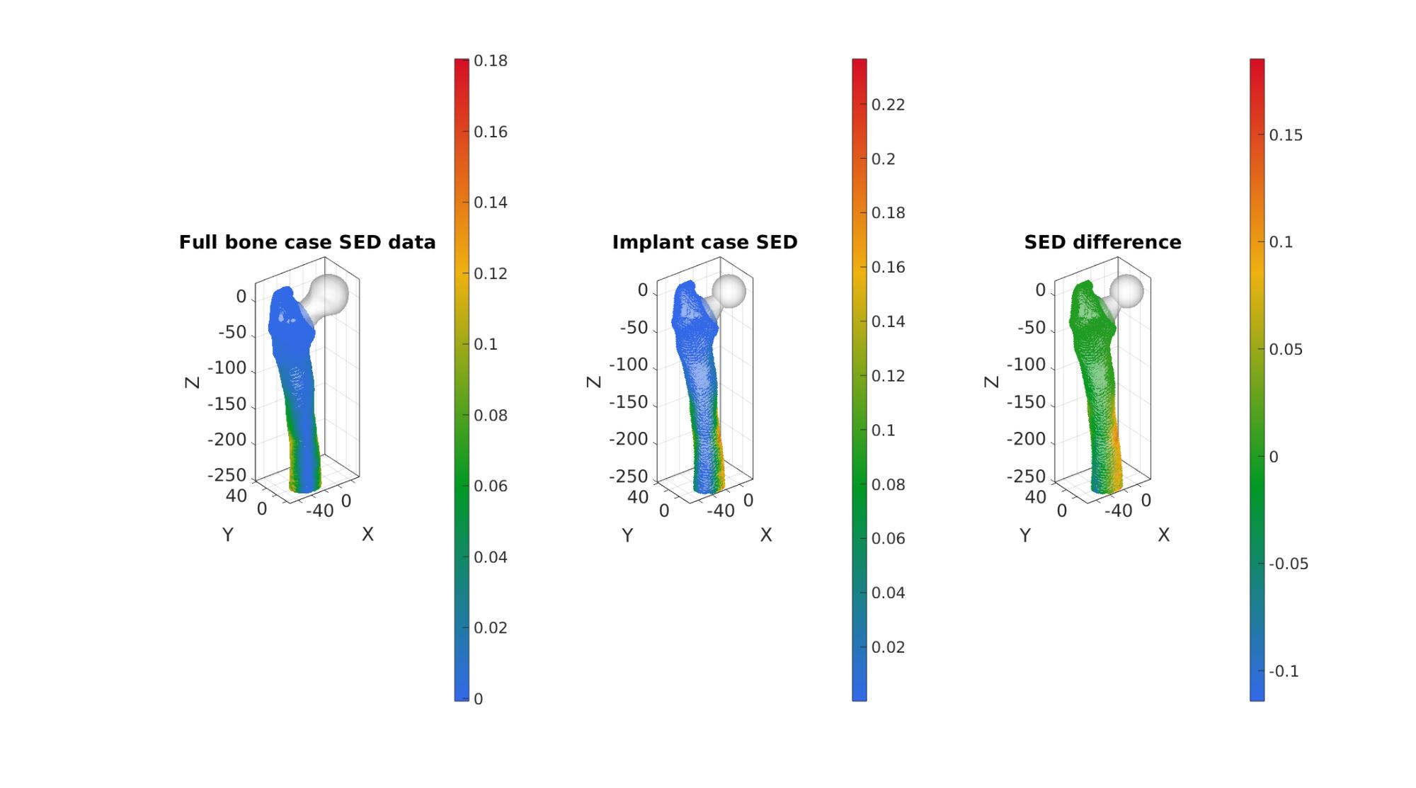
Compare to non-implant case

    if skipCompare==0

        % Interpolate at coordinates with implant
        W_p_at_VE_12=interpFuncEnergy(VE_12);

        W_12=E_energy(logicBoneElements,:,end); %SED for all elements

        delta_W=W_12-W_p_at_VE_12; %Energy difference between cases

        %Sum of squared delta_W
        delta_W_ssqd=sum(delta_W.^2);

        cFigure;

        subplot(1,3,1); hold on;
        title('Full bone case SED data');
        gpatch(Fb_no_implant,V_no_implant,'w','none',0.5); %Add graphics object to animate
        scatterV(VE_12,50,W_p_at_VE_12,'filled');
        axisGeom(gca,fontSize); colormap(gjet(250)); colorbar;
        camlight headlight;

        subplot(1,3,2); hold on;
        title('Implant case SED');
        gpatch(Fb,V,'w','none',0.5); %Add graphics object to animate
        scatterV(VE_12,25,W_12,'filled');
        axisGeom(gca,fontSize); colormap(gjet(250)); colorbar;
        camlight headlight;

        subplot(1,3,3); hold on;
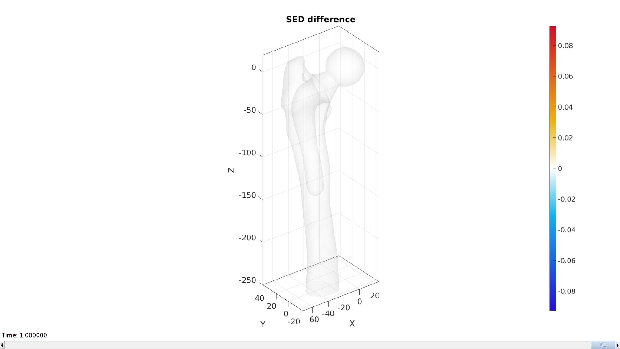
        title('SED difference');
        gpatch(Fb,V,'w','none',0.5); %Add graphics object to animate
        %     gpatch(Fb_p,V_p,'w','none',0.5); %Add graphics object to animate

        scatterV(VE_12,25,delta_W,'filled');

        axisGeom(gca,fontSize); colormap(gjet(250)); colorbar;
        camlight headlight;
        drawnow;

        C_data=delta_W;

        n=[0 1 0]; %Normal direction to plane
        P=mean(V,1); %Point on plane
        [logicAt]=meshCleave(E_12,V,P,n);

        % Get faces and matching color data for visualization
        [F_cleave,CF_cleave]=element2patch(E_12(logicAt,:),C_data(logicAt));

        hf=cFigure; hold on;
        title('SED difference');
        gpatch(Fb,V,'w','none',0.1); %Add graphics object to animate

        hp1=gpatch(F_cleave,V,CF_cleave,'k',1);
        axisGeom(gca,fontSize);
        colormap(warmcold(250));
        caxis([-(max(abs(C_data))) (max(abs(C_data)))]/2);
        axis(axisLim(V_DEF)); %Set axis limits statically
        colorbar; axis manual;
        camlight headligth;
        gdrawnow;

        nSteps=25; %Number of animation steps

        %Create the time vector
        animStruct.Time=linspace(0,1,nSteps);

        %The vector lengths
        y=linspace(min(V(:,2)),max(V(:,2)),nSteps);
        for q=1:1:nSteps

            logicAt=meshCleave(E_12,V,[0 y(q) 0],n,[1 0]);

            % Get faces and matching color data for cleaves elements
            [F_cleave,CF_cleave]=element2patch(E_12(logicAt,:),C_data(logicAt));

            %Set entries in animation structure
            animStruct.Handles{q}=[hp1 hp1]; %Handles of objects to animate
            animStruct.Props{q}={'Faces','CData'}; %Properties of objects to animate
            animStruct.Set{q}={F_cleave,CF_cleave}; %Property values for to set in order to animate
        end
        anim8(hf,animStruct);

end

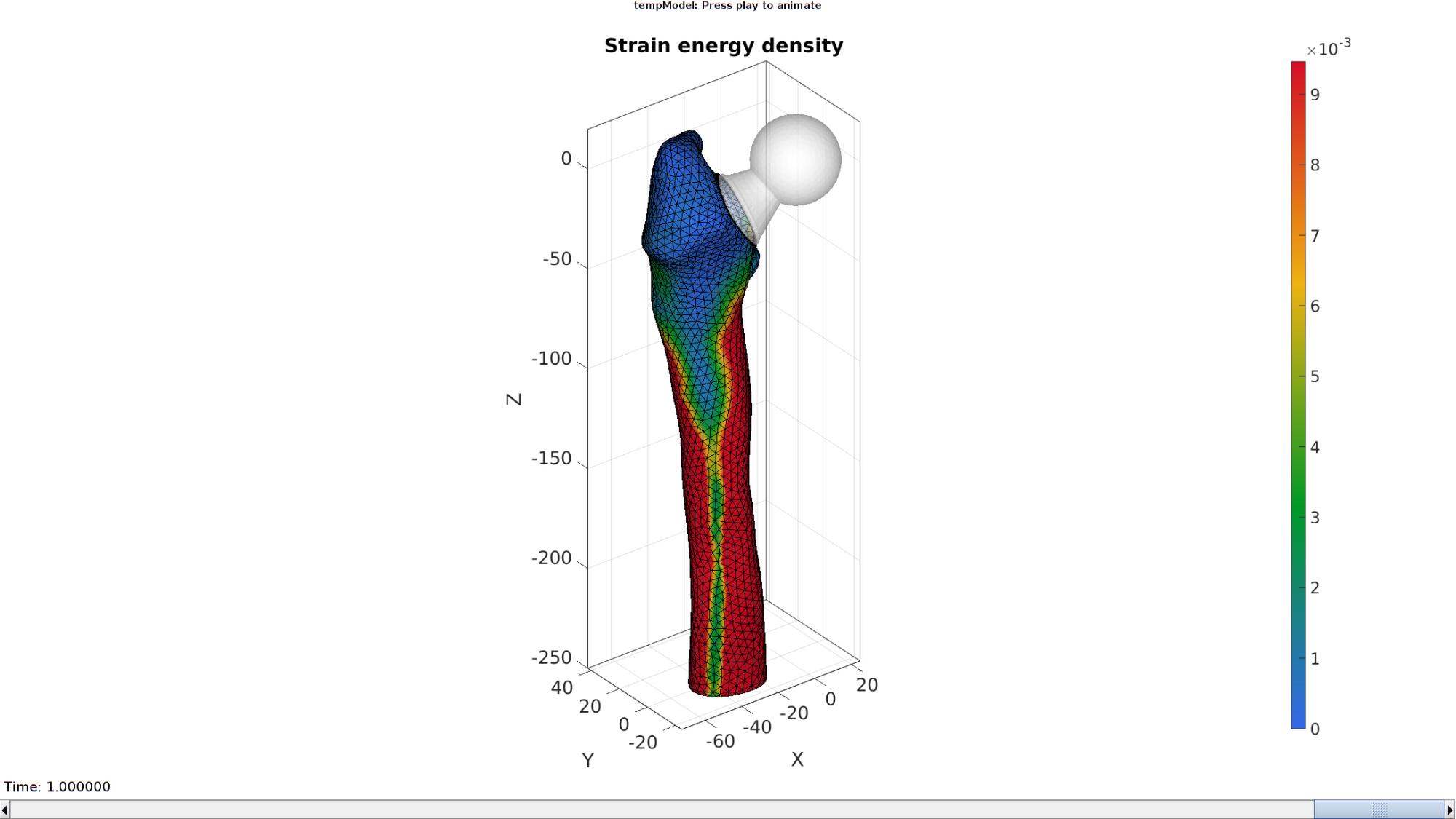
simulated results using `anim8` to visualize and animate

deformations

    FE_face=element2patch(E_12,[],'tet4');
    [indBoundary]=tesBoundary(FE_face);
    Fb_energy=FE_face(indBoundary,:);

    [CV]=faceToVertexMeasure(E_12,V,E_energy(logicBoneElements,:,end));

    % Create basic view and store graphics handle to initiate animation
    hf=cFigure; %Open figure
    title('Strain energy density')
    gtitle([febioFebFileNamePart,': Press play to animate']);

    hp1=gpatch(Fb(Cb>3,:),V_DEF(:,:,end),'w','none',0.5); %Add graphics object to animate
    hp2=gpatch(Fb_energy,V_DEF(:,:,end),CV,'k',1); %Add graphics object to animate
    hp2.FaceColor='Interp';

    axisGeom(gca,fontSize);
    colormap(gjet(250)); colorbar;
    caxis([0 max(E_energy(:))/25]);
    axis(axisLim(V_DEF)); %Set axis limits statically
    camlight headlight;

    % Set up animation features
    animStruct.Time=timeVec; %The time vector
    for qt=1:1:size(N_disp_mat,3) %Loop over time increments
        DN=N_disp_mat(:,:,qt); %Current disp

        [CV]=faceToVertexMeasure(E_12,V,E_energy(logicBoneElements,:,qt));

        %Set entries in animation structure
        animStruct.Handles{qt}=[hp1 hp2 hp2]; %Handles of objects to animate
        animStruct.Props{qt}={'Vertices','Vertices','CData'}; %Properties of objects to animate
        animStruct.Set{qt}={V_DEF(:,:,qt),V_DEF(:,:,qt),CV}; %Property values for to set in order to animate
    end
    anim8(hf,animStruct); %Initiate animation feature
    drawnow;

end

GIBBON footer text

License: https://github.com/gibbonCode/GIBBON/blob/master/LICENSE

GIBBON: The Geometry and Image-based Bioengineering add-On. A toolbox for image segmentation, image-based modeling, meshing, and finite element analysis.

This program is free software: you can redistribute it and/or modify it under the terms of the GNU General Public License as published by the Free Software Foundation, either version 3 of the License, or (at your option) any later version.

This program is distributed in the hope that it will be useful, but WITHOUT ANY WARRANTY; without even the implied warranty of MERCHANTABILITY or FITNESS FOR A PARTICULAR PURPOSE. See the GNU General Public License for more details.

You should have received a copy of the GNU General Public License along with this program. If not, see http://www.gnu.org/licenses/.