DEMO_febio_0001_cube_uniaxial

Below is a demonstration for:

Building geometry for a cube with hexahedral elements
Defining the boundary conditions
Coding the febio structure
Running the model
Importing and visualizing the displacement and stress results

Keywords
Plot settings
Control parameters
Creating model geometry and mesh
Defining the boundary conditions
Defining the FEBio input structure
Quick viewing of the FEBio input file structure
Exporting the FEBio input file
Running the FEBio analysis
Import FEBio results

Keywords

febio_spec version 4.0
febio, FEBio
uniaxial loading
compression, tension, compressive, tensile
displacement control, displacement boundary condition
hexahedral elements, hex8
cube, box, rectangular
static, solid
neo-hookean, uncoupled
displacement logfile
stress logfile

clear; close all; clc;

Plot settings

fontSize=20;
faceAlpha1=0.8;
markerSize=40;
markerSize2=35;
lineWidth=3;
cMap=viridis(20); %colormap

Control parameters

% Path names
defaultFolder = fileparts(fileparts(mfilename('fullpath')));
savePath=fullfile(defaultFolder,'data','temp');

% Defining file names
febioFebFileNamePart='tempModel';
febioFebFileName=fullfile(savePath,[febioFebFileNamePart,'.feb']); %FEB file name
febioLogFileName=[febioFebFileNamePart,'.txt']; %FEBio log file name
febioLogFileName_disp=[febioFebFileNamePart,'_disp_out.txt']; %Log file name for exporting displacement
febioLogFileName_stress=[febioFebFileNamePart,'_stress_out.txt']; %Log file name for exporting stress sigma_z
febioLogFileName_stretch=[febioFebFileNamePart,'_stretch_out.txt']; %Log file name for exporting stretch U_z
febioLogFileName_stress_prin=[febioFebFileNamePart,'_stress_prin_out.txt']; %Log file name for exporting principal stresses
febioLogFileName_stretch_prin=[febioFebFileNamePart,'_stretch_prin_out.txt']; %Log file name for exporting principal stretches
febioLogFileName_force=[febioFebFileNamePart,'_force_out.txt']; %Log file name for exporting force

%Specifying dimensions and number of elements
cubeSize=10;
sampleWidth=cubeSize; %Width
sampleThickness=cubeSize; %Thickness
sampleHeight=cubeSize; %Height
pointSpacings=2*ones(1,3); %Desired point spacing between nodes
numElementsWidth=round(sampleWidth/pointSpacings(1)); %Number of elemens in dir 1
numElementsThickness=round(sampleThickness/pointSpacings(2)); %Number of elemens in dir 2
numElementsHeight=round(sampleHeight/pointSpacings(3)); %Number of elemens in dir 3

%Define applied displacement
appliedStrain=0.3; %Linear strain (Only used to compute applied stretch)
loadingOption='compression'; % or 'tension'
switch loadingOption
    case 'compression'
        stretchLoad=1-appliedStrain; %The applied stretch for uniaxial loading
    case 'tension'
        stretchLoad=1+appliedStrain; %The applied stretch for uniaxial loading
end
displacementMagnitude=(stretchLoad*sampleHeight)-sampleHeight; %The displacement magnitude

%Material parameter set
E_youngs1=0.1; %Material Young's modulus
nu1=0.4; %Material Poisson's ratio

% FEA control settings
numTimeSteps=10; %Number of time steps desired
max_refs=25; %Max reforms
max_ups=0; %Set to zero to use full-Newton iterations
opt_iter=6; %Optimum number of iterations
max_retries=5; %Maximum number of retires
dtmin=(1/numTimeSteps)/100; %Minimum time step size
dtmax=1/numTimeSteps; %Maximum time step size

runMode='external';% 'internal' or 'external'

Creating model geometry and mesh

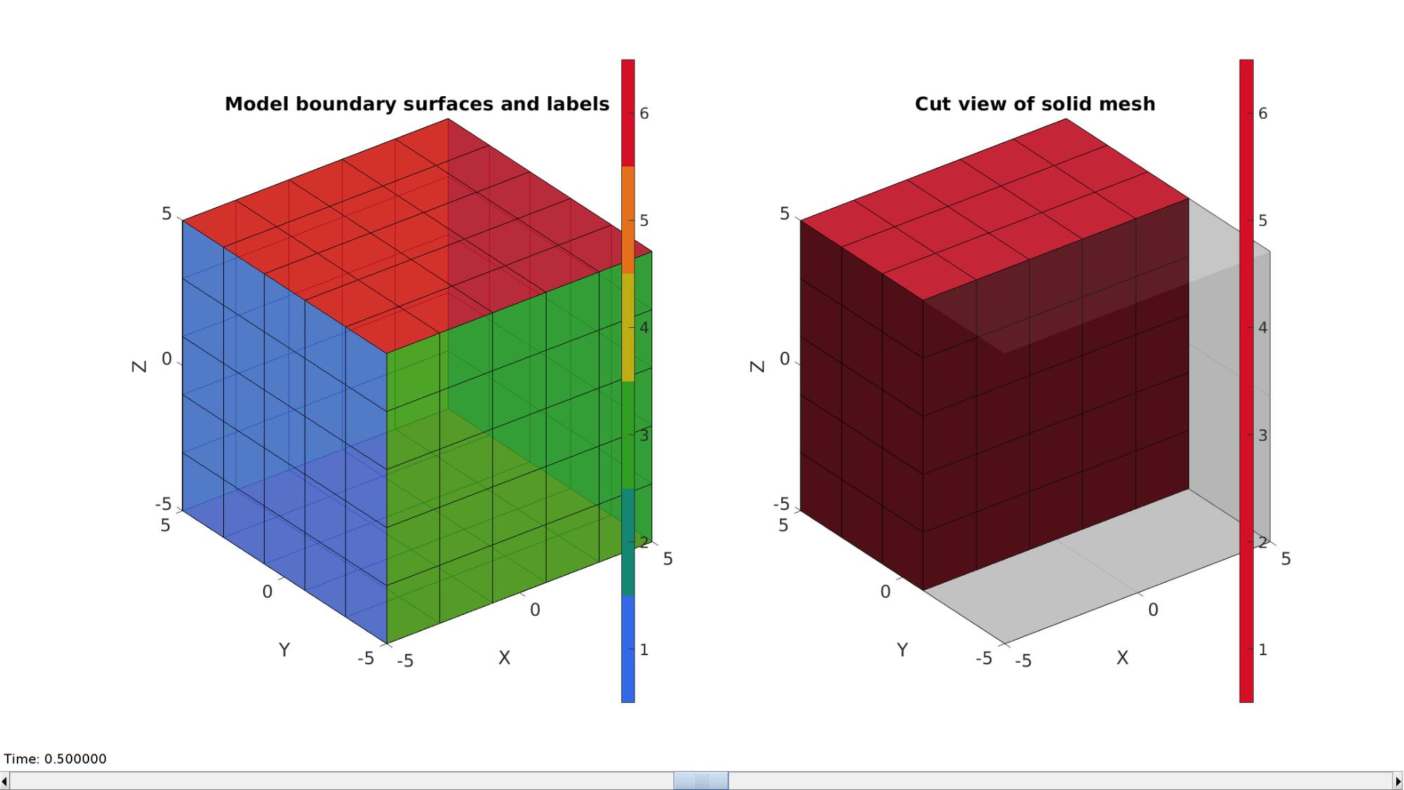
A box is created with tri-linear hexahedral (hex8) elements using the hexMeshBox function. The function offers the boundary faces with seperate labels for the top, bottom, left, right, front, and back sides. As such these can be used to define boundary conditions on the exterior.

% Create a box with hexahedral elements
cubeDimensions=[sampleWidth sampleThickness sampleHeight]; %Dimensions
cubeElementNumbers=[numElementsWidth numElementsThickness numElementsHeight]; %Number of elements
outputStructType=2; %A structure compatible with mesh view
[meshStruct]=hexMeshBox(cubeDimensions,cubeElementNumbers,outputStructType);

%Access elements, nodes, and faces from the structure
E=meshStruct.elements; %The elements
V=meshStruct.nodes; %The nodes (vertices)
Fb=meshStruct.facesBoundary; %The boundary faces
Cb=meshStruct.boundaryMarker; %The "colors" or labels for the boundary faces
elementMaterialIndices=ones(size(E,1),1); %Element material indices

Plotting model boundary surfaces and a cut view

hFig=cFigure;

subplot(1,2,1); hold on;
title('Model boundary surfaces and labels','FontSize',fontSize);
gpatch(Fb,V,Cb,'k',faceAlpha1);
colormap(gjet(6)); icolorbar;
axisGeom(gca,fontSize);

hs=subplot(1,2,2); hold on;
title('Cut view of solid mesh','FontSize',fontSize);
optionStruct.hFig=[hFig hs];
meshView(meshStruct,optionStruct);
axisGeom(gca,fontSize);

drawnow;

Defining the boundary conditions

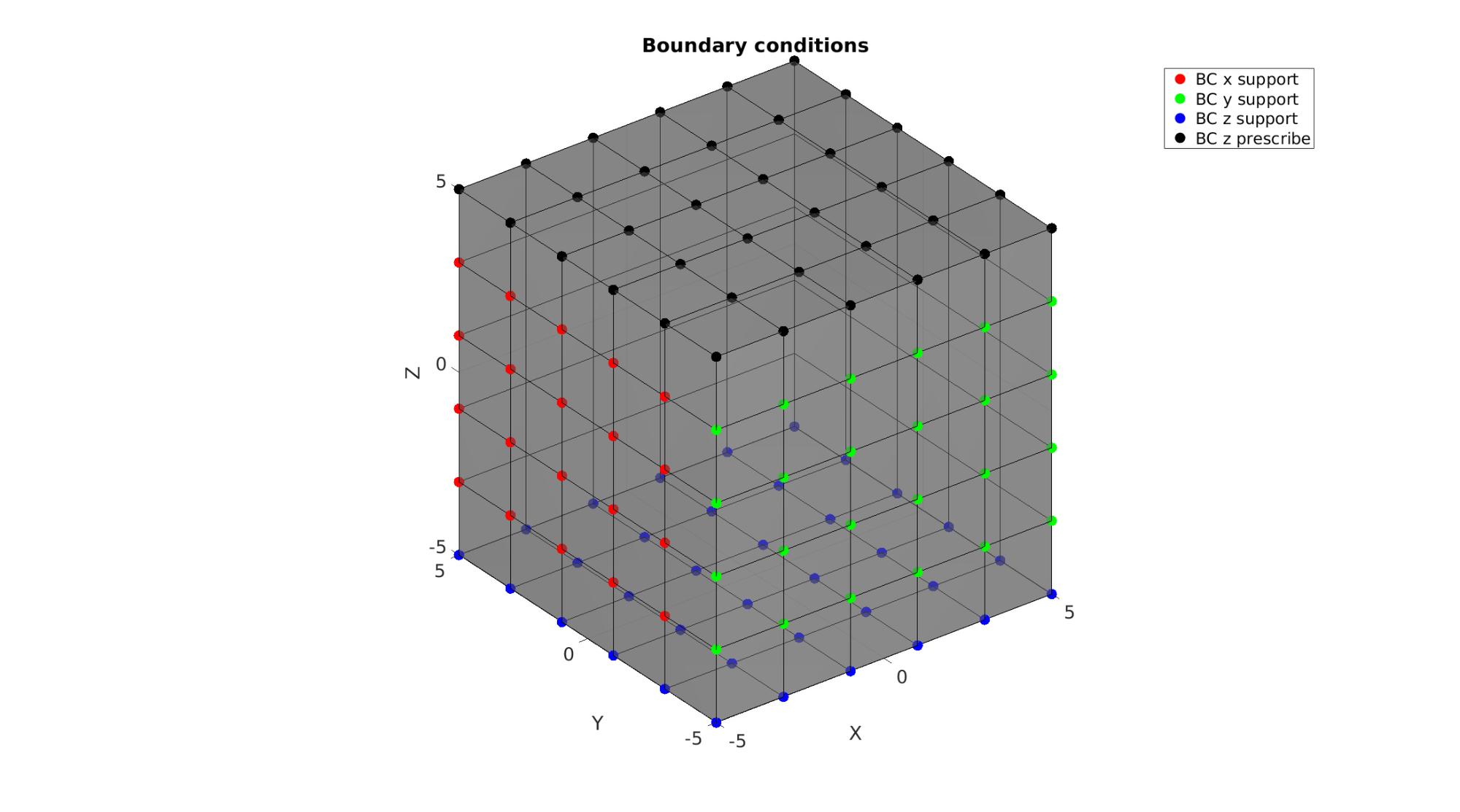
The visualization of the model boundary shows colors for each side of the cube. These labels can be used to define boundary conditions.

%Define supported node sets
logicFace=Cb==1; %Logic for current face set
Fr=Fb(logicFace,:); %The current face set
bcSupportList_X=unique(Fr(:)); %Node set part of selected face

logicFace=Cb==3; %Logic for current face set
Fr=Fb(logicFace,:); %The current face set
bcSupportList_Y=unique(Fr(:)); %Node set part of selected face

logicFace=Cb==5; %Logic for current face set
Fr=Fb(logicFace,:); %The current face set
bcSupportList_Z=unique(Fr(:)); %Node set part of selected face

%Prescribed displacement nodes
logicPrescribe=Cb==6; %Logic for current face set
Fr=Fb(logicPrescribe,:); %The current face set
bcPrescribeList=unique(Fr(:)); %Node set part of selected face

Visualizing boundary conditions. Markers plotted on the semi-transparent model denote the nodes in the various boundary condition lists.

hf=cFigure;
title('Boundary conditions','FontSize',fontSize);
xlabel('X','FontSize',fontSize); ylabel('Y','FontSize',fontSize); zlabel('Z','FontSize',fontSize);
hold on;

gpatch(Fb,V,'kw','k',0.5);

hl(1)=plotV(V(bcSupportList_X,:),'r.','MarkerSize',markerSize);
hl(2)=plotV(V(bcSupportList_Y,:),'g.','MarkerSize',markerSize);
hl(3)=plotV(V(bcSupportList_Z,:),'b.','MarkerSize',markerSize);
hl(4)=plotV(V(bcPrescribeList,:),'k.','MarkerSize',markerSize);

legend(hl,{'BC x support','BC y support','BC z support','BC z prescribe'});

axisGeom(gca,fontSize);
camlight headlight;
drawnow;

Defining the FEBio input structure

See also febioStructTemplate and febioStruct2xml and the FEBio user manual.

%Get a template with default settings
[febio_spec]=febioStructTemplate;

%febio_spec version
febio_spec.ATTR.version='4.0';

%Module section
febio_spec.Module.ATTR.type='solid';

%Control section
febio_spec.Control.analysis='STATIC';
febio_spec.Control.time_steps=numTimeSteps;
febio_spec.Control.step_size=1/numTimeSteps;
febio_spec.Control.solver.max_refs=max_refs;
febio_spec.Control.solver.qn_method.max_ups=max_ups;
febio_spec.Control.time_stepper.dtmin=dtmin;
febio_spec.Control.time_stepper.dtmax=dtmax;
febio_spec.Control.time_stepper.max_retries=max_retries;
febio_spec.Control.time_stepper.opt_iter=opt_iter;

%Material section
materialName1='Material1';
febio_spec.Material.material{1}.ATTR.name=materialName1;
febio_spec.Material.material{1}.ATTR.type='neo-Hookean';
febio_spec.Material.material{1}.ATTR.id=1;
febio_spec.Material.material{1}.E=E_youngs1;
febio_spec.Material.material{1}.v=nu1;

% Mesh section
% -> Nodes
febio_spec.Mesh.Nodes{1}.ATTR.name='Object1'; %The node set name
febio_spec.Mesh.Nodes{1}.node.ATTR.id=(1:size(V,1))'; %The node id's
febio_spec.Mesh.Nodes{1}.node.VAL=V; %The nodel coordinates

% -> Elements
partName1='Part1';
febio_spec.Mesh.Elements{1}.ATTR.name=partName1; %Name of this part
febio_spec.Mesh.Elements{1}.ATTR.type='hex8'; %Element type
febio_spec.Mesh.Elements{1}.elem.ATTR.id=(1:1:size(E,1))'; %Element id's
febio_spec.Mesh.Elements{1}.elem.VAL=E; %The element matrix

% -> NodeSets
nodeSetName1='bcSupportList_X';
nodeSetName2='bcSupportList_Y';
nodeSetName3='bcSupportList_Z';
nodeSetName4='bcPrescribeList';

febio_spec.Mesh.NodeSet{1}.ATTR.name=nodeSetName1;
febio_spec.Mesh.NodeSet{1}.VAL=mrow(bcSupportList_X);

febio_spec.Mesh.NodeSet{2}.ATTR.name=nodeSetName2;
febio_spec.Mesh.NodeSet{2}.VAL=mrow(bcSupportList_Y);

febio_spec.Mesh.NodeSet{3}.ATTR.name=nodeSetName3;
febio_spec.Mesh.NodeSet{3}.VAL=mrow(bcSupportList_Z);

febio_spec.Mesh.NodeSet{4}.ATTR.name=nodeSetName4;
febio_spec.Mesh.NodeSet{4}.VAL=mrow(bcPrescribeList);

%MeshDomains section
febio_spec.MeshDomains.SolidDomain.ATTR.name=partName1;
febio_spec.MeshDomains.SolidDomain.ATTR.mat=materialName1;

%Boundary condition section
% -> Fix boundary conditions
febio_spec.Boundary.bc{1}.ATTR.name='zero_displacement_x';
febio_spec.Boundary.bc{1}.ATTR.type='zero displacement';
febio_spec.Boundary.bc{1}.ATTR.node_set=nodeSetName1;
febio_spec.Boundary.bc{1}.x_dof=1;
febio_spec.Boundary.bc{1}.y_dof=0;
febio_spec.Boundary.bc{1}.z_dof=0;

febio_spec.Boundary.bc{2}.ATTR.name='zero_displacement_y';
febio_spec.Boundary.bc{2}.ATTR.type='zero displacement';
febio_spec.Boundary.bc{2}.ATTR.node_set=nodeSetName2;
febio_spec.Boundary.bc{2}.x_dof=0;
febio_spec.Boundary.bc{2}.y_dof=1;
febio_spec.Boundary.bc{2}.z_dof=0;

febio_spec.Boundary.bc{3}.ATTR.name='zero_displacement_z';
febio_spec.Boundary.bc{3}.ATTR.type='zero displacement';
febio_spec.Boundary.bc{3}.ATTR.node_set=nodeSetName3;
febio_spec.Boundary.bc{3}.x_dof=0;
febio_spec.Boundary.bc{3}.y_dof=0;
febio_spec.Boundary.bc{3}.z_dof=1;

febio_spec.Boundary.bc{4}.ATTR.name='prescibed_displacement_z';
febio_spec.Boundary.bc{4}.ATTR.type='prescribed displacement';
febio_spec.Boundary.bc{4}.ATTR.node_set=nodeSetName4;
febio_spec.Boundary.bc{4}.dof='z';
febio_spec.Boundary.bc{4}.value.ATTR.lc=1;
febio_spec.Boundary.bc{4}.value.VAL=displacementMagnitude;
febio_spec.Boundary.bc{4}.relative=0;

%LoadData section
% -> load_controller
febio_spec.LoadData.load_controller{1}.ATTR.name='LC_1';
febio_spec.LoadData.load_controller{1}.ATTR.id=1;
febio_spec.LoadData.load_controller{1}.ATTR.type='loadcurve';
febio_spec.LoadData.load_controller{1}.interpolate='LINEAR';
%febio_spec.LoadData.load_controller{1}.extend='CONSTANT';
febio_spec.LoadData.load_controller{1}.points.pt.VAL=[0 0; 1 1];

%Output section
% -> log file
febio_spec.Output.logfile.ATTR.file=febioLogFileName;
febio_spec.Output.logfile.node_data{1}.ATTR.file=febioLogFileName_disp;
febio_spec.Output.logfile.node_data{1}.ATTR.data='ux;uy;uz';
febio_spec.Output.logfile.node_data{1}.ATTR.delim=',';

febio_spec.Output.logfile.node_data{2}.ATTR.file=febioLogFileName_force;
febio_spec.Output.logfile.node_data{2}.ATTR.data='Rx;Ry;Rz';
febio_spec.Output.logfile.node_data{2}.ATTR.delim=',';

febio_spec.Output.logfile.element_data{1}.ATTR.file=febioLogFileName_stress;
febio_spec.Output.logfile.element_data{1}.ATTR.data='sz';
febio_spec.Output.logfile.element_data{1}.ATTR.delim=',';

febio_spec.Output.logfile.element_data{2}.ATTR.file=febioLogFileName_stretch;
febio_spec.Output.logfile.element_data{2}.ATTR.data='Uz';
febio_spec.Output.logfile.element_data{2}.ATTR.delim=',';

febio_spec.Output.logfile.element_data{3}.ATTR.file=febioLogFileName_stress_prin;
febio_spec.Output.logfile.element_data{3}.ATTR.data='s1;s2;s3';
febio_spec.Output.logfile.element_data{3}.ATTR.delim=',';

febio_spec.Output.logfile.element_data{4}.ATTR.file=febioLogFileName_stretch_prin;
febio_spec.Output.logfile.element_data{4}.ATTR.data='U1;U2;U3';
febio_spec.Output.logfile.element_data{4}.ATTR.delim=',';

% Plotfile section
febio_spec.Output.plotfile.compression=0;

Quick viewing of the FEBio input file structure

The febView function can be used to view the xml structure in a MATLAB figure window.

febView(febio_spec); %Viewing the febio file

Exporting the FEBio input file

Exporting the febio_spec structure to an FEBio input file is done using the febioStruct2xml function.

febioStruct2xml(febio_spec,febioFebFileName); %Exporting to file and domNode
%system(['gedit ',febioFebFileName,' &']);

Running the FEBio analysis

To run the analysis defined by the created FEBio input file the runMonitorFEBio function is used. The input for this function is a structure defining job settings e.g. the FEBio input file name. The optional output runFlag informs the user if the analysis was run succesfully.

febioAnalysis.run_filename=febioFebFileName; %The input file name
febioAnalysis.run_logname=febioLogFileName; %The name for the log file
febioAnalysis.disp_on=1; %Display information on the command window
febioAnalysis.runMode=runMode;
febioAnalysis.maxLogCheckTime=10; %Max log file checking time

[runFlag]=runMonitorFEBio(febioAnalysis);%START FEBio NOW!!!!!!!!

 
%%%%%%%%%%%%%%%%%%%%%%%%%%%%%%%%%%%%%%%%%%%%%%%%%%%%%%%%%%%%%%%%%%%%%%%%%%%
-------->    RUNNING/MONITORING FEBIO JOB    <-------- 27-Apr-2023 10:20:56
FEBio path: /home/kevin/FEBioStudio2/bin/febio4
# Attempt removal of existing log files                27-Apr-2023 10:20:56
 * Removal succesful                                   27-Apr-2023 10:20:56
# Attempt removal of existing .xplt files              27-Apr-2023 10:20:56
 * Removal succesful                                   27-Apr-2023 10:20:56
# Starting FEBio...                                    27-Apr-2023 10:20:56
  Max. total analysis time is: Inf s
 * Waiting for log file creation                       27-Apr-2023 10:20:56
   Max. wait time: 10 s
 * Log file found.                                     27-Apr-2023 10:20:56
# Parsing log file...                                  27-Apr-2023 10:20:56
    number of iterations   : 3                         27-Apr-2023 10:20:57
    number of reformations : 3                         27-Apr-2023 10:20:57
------- converged at time : 0.1                        27-Apr-2023 10:20:57
    number of iterations   : 3                         27-Apr-2023 10:20:57
    number of reformations : 3                         27-Apr-2023 10:20:57
------- converged at time : 0.2                        27-Apr-2023 10:20:57
    number of iterations   : 3                         27-Apr-2023 10:20:57
    number of reformations : 3                         27-Apr-2023 10:20:57
------- converged at time : 0.3                        27-Apr-2023 10:20:57
    number of iterations   : 3                         27-Apr-2023 10:20:57
    number of reformations : 3                         27-Apr-2023 10:20:57
------- converged at time : 0.4                        27-Apr-2023 10:20:57
    number of iterations   : 3                         27-Apr-2023 10:20:57
    number of reformations : 3                         27-Apr-2023 10:20:57
------- converged at time : 0.5                        27-Apr-2023 10:20:57
    number of iterations   : 3                         27-Apr-2023 10:20:57
    number of reformations : 3                         27-Apr-2023 10:20:57
------- converged at time : 0.6                        27-Apr-2023 10:20:57
    number of iterations   : 3                         27-Apr-2023 10:20:57
    number of reformations : 3                         27-Apr-2023 10:20:57
------- converged at time : 0.7                        27-Apr-2023 10:20:57
    number of iterations   : 3                         27-Apr-2023 10:20:57
    number of reformations : 3                         27-Apr-2023 10:20:57
------- converged at time : 0.8                        27-Apr-2023 10:20:57
    number of iterations   : 3                         27-Apr-2023 10:20:57
    number of reformations : 3                         27-Apr-2023 10:20:57
------- converged at time : 0.9                        27-Apr-2023 10:20:57
    number of iterations   : 3                         27-Apr-2023 10:20:57
    number of reformations : 3                         27-Apr-2023 10:20:57
------- converged at time : 1                          27-Apr-2023 10:20:57
 Elapsed time : 0:00:00                                27-Apr-2023 10:20:57
 N O R M A L   T E R M I N A T I O N
# Done                                                 27-Apr-2023 10:20:57
%%%%%%%%%%%%%%%%%%%%%%%%%%%%%%%%%%%%%%%%%%%%%%%%%%%%%%%%%%%%%%%%%%%%%%%%%%%

Import FEBio results

if runFlag==1 %i.e. a succesful run

    % Importing nodal displacements from a log file
    dataStruct=importFEBio_logfile(fullfile(savePath,febioLogFileName_disp),0,1);

    %Access data
    N_disp_mat=dataStruct.data; %Displacement
    timeVec=dataStruct.time; %Time

    %Create deformed coordinate set
    V_DEF=N_disp_mat+repmat(V,[1 1 size(N_disp_mat,3)]);

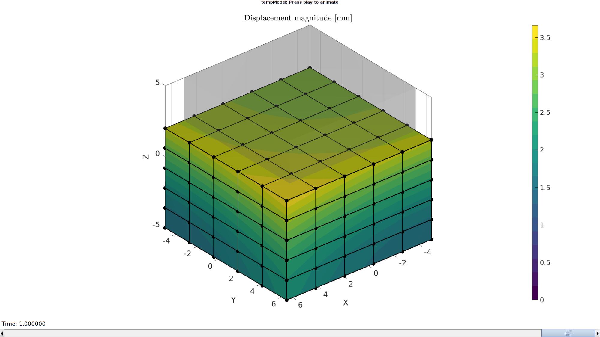
Plotting the simulated results using anim8 to visualize and animate deformations

    DN_magnitude=sqrt(sum(N_disp_mat(:,:,end).^2,2)); %Current displacement magnitude

    % Create basic view and store graphics handle to initiate animation
    hf=cFigure; %Open figure
    gtitle([febioFebFileNamePart,': Press play to animate']);
    title('Displacement magnitude [mm]','Interpreter','Latex')
    hp=gpatch(Fb,V_DEF(:,:,end),DN_magnitude,'k',1,2); %Add graphics object to animate
    hp.Marker='.';
    hp.MarkerSize=markerSize2;
    hp.FaceColor='interp';
    gpatch(Fb,V,0.5*ones(1,3),'none',0.25); %A static graphics object

    axisGeom(gca,fontSize);
    colormap(cMap); colorbar;
    caxis([0 max(DN_magnitude)]); caxis manual;
    axis(axisLim(V_DEF)); %Set axis limits statically
    view(140,30);
    camlight headlight;

    % Set up animation features
    animStruct.Time=timeVec; %The time vector
    for qt=1:1:size(N_disp_mat,3) %Loop over time increments
        DN_magnitude=sqrt(sum(N_disp_mat(:,:,qt).^2,2)); %Current displacement magnitude

        %Set entries in animation structure
        animStruct.Handles{qt}=[hp hp]; %Handles of objects to animate
        animStruct.Props{qt}={'Vertices','CData'}; %Properties of objects to animate
        animStruct.Set{qt}={V_DEF(:,:,qt),DN_magnitude}; %Property values for to set in order to animate
    end
    anim8(hf,animStruct); %Initiate animation feature
    drawnow;

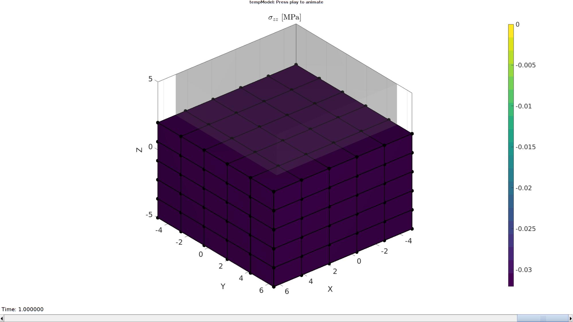
Importing element stress from a log file

    dataStruct=importFEBio_logfile(fullfile(savePath,febioLogFileName_stress),0,1);

    %Access data
    E_stress_mat=dataStruct.data;

Importing element stretch from a log file

    dataStruct=importFEBio_logfile(fullfile(savePath,febioLogFileName_stretch),0,1);

    %Access data
    E_stretch_mat=dataStruct.data;

Plotting the simulated results using anim8 to visualize and animate deformations

    [CV]=faceToVertexMeasure(E,V,E_stress_mat(:,:,end));

    % Create basic view and store graphics handle to initiate animation
    hf=cFigure; %Open figure  /usr/local/MATLAB/R2020a/bin/glnxa64/jcef_helper: symbol lookup error: /lib/x86_64-linux-gnu/libpango-1.0.so.0: undefined symbol: g_ptr_array_copy

    gtitle([febioFebFileNamePart,': Press play to animate']);
    title('$\sigma_{zz}$ [MPa]','Interpreter','Latex')
    hp=gpatch(Fb,V_DEF(:,:,end),CV,'k',1,2); %Add graphics object to animate
    hp.Marker='.';
    hp.MarkerSize=markerSize2;
    hp.FaceColor='interp';
    gpatch(Fb,V,0.5*ones(1,3),'none',0.25); %A static graphics object

    axisGeom(gca,fontSize);
    colormap(cMap); colorbar;
    caxis([min(E_stress_mat(:)) max(E_stress_mat(:))]);
    axis(axisLim(V_DEF)); %Set axis limits statically
    view(140,30);
    camlight headlight;

    % Set up animation features
    animStruct.Time=timeVec; %The time vector
    for qt=1:1:size(N_disp_mat,3) %Loop over time increments

        [CV]=faceToVertexMeasure(E,V,E_stress_mat(:,:,qt));

        %Set entries in animation structure
        animStruct.Handles{qt}=[hp hp]; %Handles of objects to animate
        animStruct.Props{qt}={'Vertices','CData'}; %Properties of objects to animate
        animStruct.Set{qt}={V_DEF(:,:,qt),CV}; %Property values for to set in order to animate
    end
    anim8(hf,animStruct); %Initiate animation feature
    drawnow;

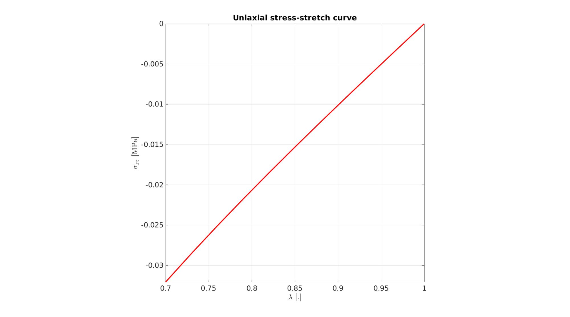
Visualize stretch-stress curve

    stretch_sim=squeeze(mean(E_stretch_mat,1)); % Stretch U_z
    stress_cauchy_sim=squeeze(mean(E_stress_mat,1)); %Cauchy stress sigma_z

    cFigure; hold on;
    title('Uniaxial stress-stretch curve','FontSize',fontSize);
    xlabel('$\lambda$ [.]','FontSize',fontSize,'Interpreter','Latex');
    ylabel('$\sigma_{zz}$ [MPa]','FontSize',fontSize,'Interpreter','Latex');

    plot(stretch_sim(:),stress_cauchy_sim(:),'r-','lineWidth',lineWidth);

    view(2); axis tight;  grid on; axis square; box on;
    set(gca,'FontSize',fontSize);
    drawnow;

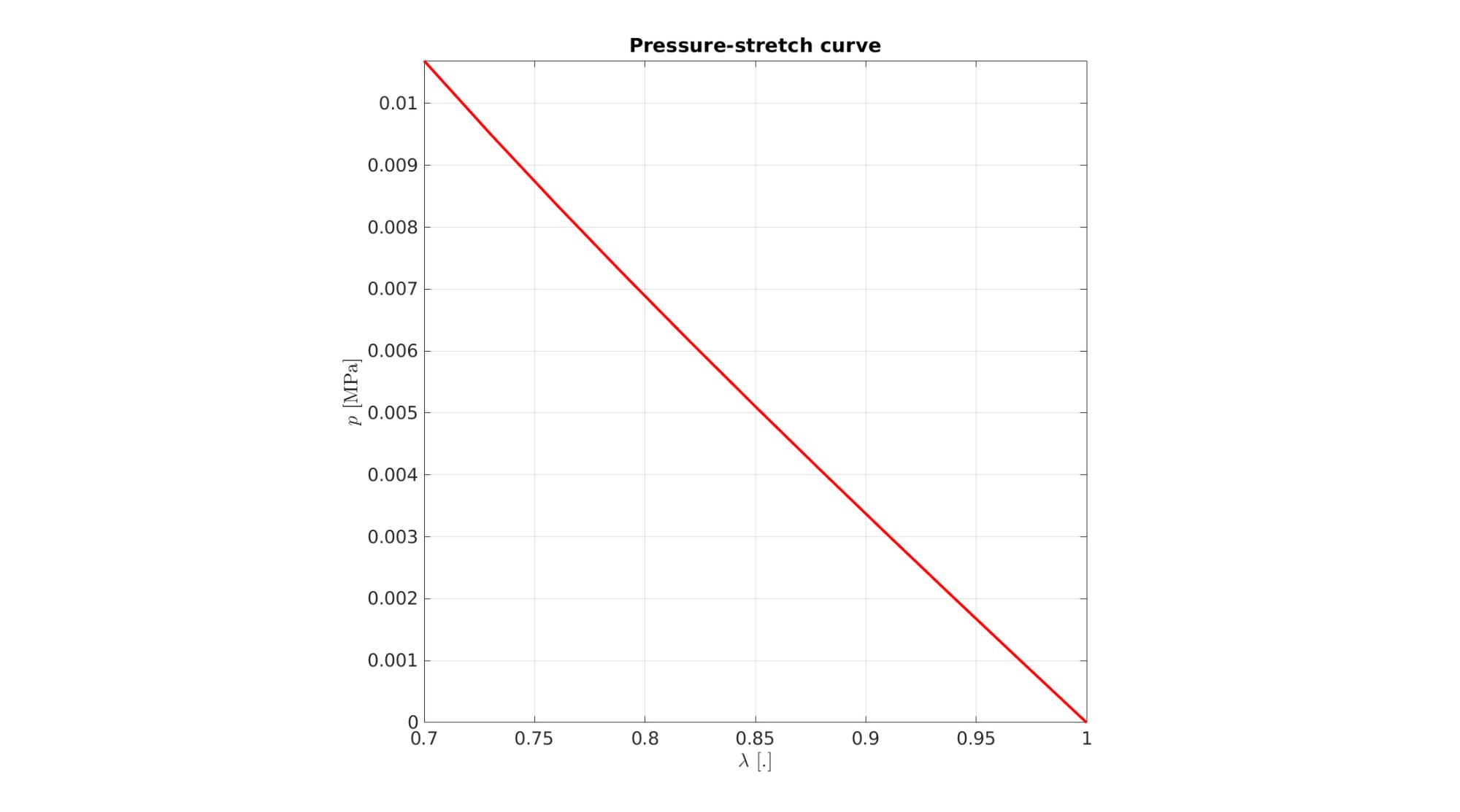
Importing element principal stresses from a log file

    dataStruct=importFEBio_logfile(fullfile(savePath,febioLogFileName_stress_prin),0,1);

    %Access data
    E_stress_prin_mat=dataStruct.data;

    %Compute pressure
    P = squeeze(-1/3*mean(sum(E_stress_prin_mat,2),1));

Visualize pressure-stretch curve

    cFigure; hold on;
    title('Pressure-stretch curve','FontSize',fontSize);
    xlabel('$\lambda$ [.]','FontSize',fontSize,'Interpreter','Latex');
    ylabel('$p$ [MPa]','FontSize',fontSize,'Interpreter','Latex');

    plot(stretch_sim(:),P(:),'r-','lineWidth',lineWidth);

    view(2); axis tight;  grid on; axis square; box on;
    set(gca,'FontSize',fontSize);
    drawnow;

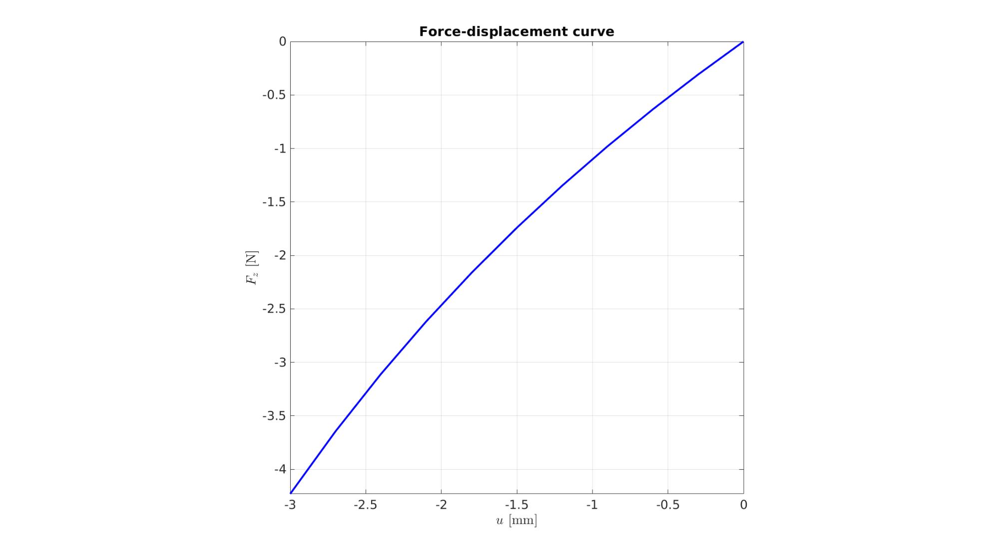
Importing nodal forces from a log file

    [dataStruct]=importFEBio_logfile(fullfile(savePath,febioLogFileName_force),0,1); %Nodal forces

    %Access data
    timeVec=dataStruct.time;
    f_sum_x=squeeze(sum(dataStruct.data(bcPrescribeList,1,:),1));
    f_sum_y=squeeze(sum(dataStruct.data(bcPrescribeList,2,:),1));
    f_sum_z=squeeze(sum(dataStruct.data(bcPrescribeList,3,:),1));

Visualize force data

    displacementApplied=timeVec.*displacementMagnitude;

    cFigure; hold on;
    title('Force-displacement curve','FontSize',fontSize);
    xlabel('$u$ [mm]','Interpreter','Latex');
    ylabel('$F_z$ [N]','Interpreter','Latex');
    hp=plot(displacementApplied(:),f_sum_z(:),'b-','LineWidth',3);
    grid on; box on; axis square; axis tight;
    set(gca,'FontSize',fontSize);
    drawnow;

end

GIBBON www.gibboncode.org

Kevin Mattheus Moerman, [email protected]

GIBBON footer text

License: https://github.com/gibbonCode/GIBBON/blob/master/LICENSE

GIBBON: The Geometry and Image-based Bioengineering add-On. A toolbox for image segmentation, image-based modeling, meshing, and finite element analysis.

This program is free software: you can redistribute it and/or modify it under the terms of the GNU General Public License as published by the Free Software Foundation, either version 3 of the License, or (at your option) any later version.

This program is distributed in the hope that it will be useful, but WITHOUT ANY WARRANTY; without even the implied warranty of MERCHANTABILITY or FITNESS FOR A PARTICULAR PURPOSE. See the GNU General Public License for more details.

You should have received a copy of the GNU General Public License along with this program. If not, see http://www.gnu.org/licenses/.